Tutorial 3: Implementing risk dynamics in the GenMR digital template

Author: Arnaud Mignan, Mignan Risk Analytics GmbH
Version: 1.2.1
Last Updated: 2026-07-23
License: AGPL-3

IN CONSTRUCTION - Please check back in late September 2026 for the official release.

A tutorial on catastrophe dynamics, demonstrating how to model chains-of-events and their cascading impacts.

• v.1.2.1 (ongoing, due Sep. 2026): Implementation of the Multi-Risk Core, consisting of the modelling of chains-of-events and risk drivers within the GenMR framework (including potentially some ad-hoc parameterisations before v.1.2.3).

• v.1.2.2 (Oct. 2026-Mar. 2027): Implementation of the generic hydropower-dam and dam flood model (led by UniL project partner) and integration into the digital template.

• v.1.2.3 (Jan. 2027-Jun. 2027): Interaction matrix encoding, with quantitative assessment of event–event and event–environment interactions within the digital template.

import numpy as np
import pandas as pd
import matplotlib.pyplot as plt

import copy
import pickle

import networkx as nx

import warnings 
warnings.filterwarnings('ignore')   # commented, try to remove all warnings

from GenMR import perils as GenMR_perils
from GenMR import environment as GenMR_env
from GenMR import dynamics as GenMR_dyn
from GenMR import utils as GenMR_utils

pd.set_option("display.max_columns", None)

# load inputs (i.e., outputs from Tutorial 1)
file_src = 'src.pkl'
file_topoLayer = 'envLayer_topo.pkl'
file_atmoLayer = 'envLayer_atmo.pkl'
file_soilLayer = 'envLayer_soil.pkl'
file_urbLandLayer = 'envLayer_urbLand.pkl'
file_energyLayer = 'envLayer_energy.pkl'
file_socioecoLayer = 'envLayer_socioeco.pkl'
file_catalog_fp_haz = 'catalog_hazFootprints.pkl'
src = GenMR_utils.load_pickle2class('/io/' + file_src)
grid = copy.copy(src.grid)
topoLayer = GenMR_utils.load_pickle2class('/io/' + file_topoLayer)
atmoLayer = GenMR_utils.load_pickle2class('/io/' + file_atmoLayer)
soilLayer = GenMR_utils.load_pickle2class('/io/' + file_soilLayer)
urbLandLayer = GenMR_utils.load_pickle2class('/io/' + file_urbLandLayer)
energyLayer = GenMR_utils.load_pickle2class('/io/' + file_energyLayer)
socioecoLayer = GenMR_utils.load_pickle2class('/io/' + file_socioecoLayer)
with open('io/' + file_catalog_fp_haz, 'rb') as f:
    catalog_fp_haz = pickle.load(f)

xmin, xmax, ymin, ymax = grid.xmin, grid.xmax, grid.ymin, grid.ymax

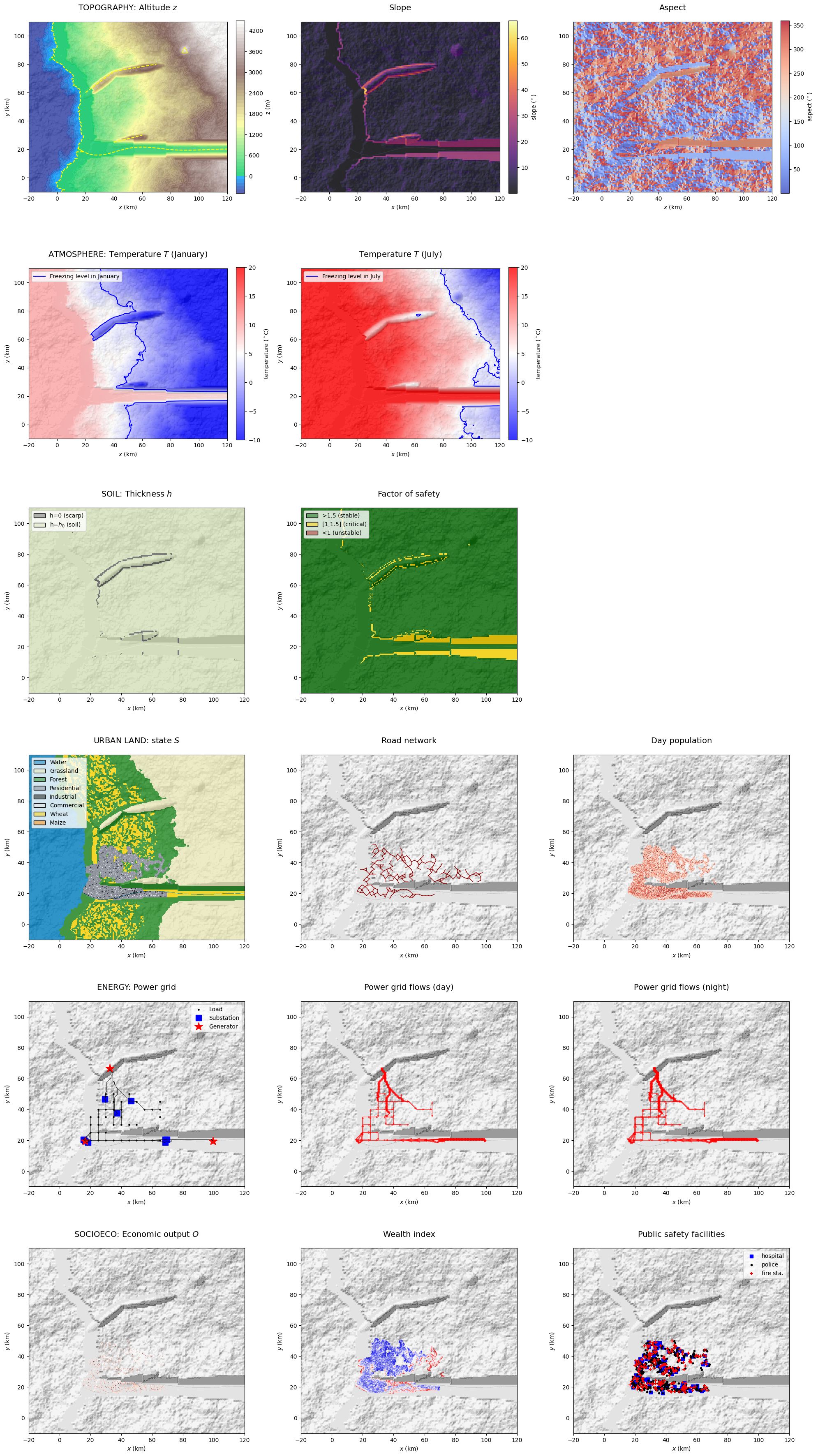
GenMR_env.plot_EnvLayers([topoLayer, atmoLayer, soilLayer, urbLandLayer, energyLayer, 
                          socioecoLayer], file_ext = 'jpg', topo_bool = True)

# load inputs (i.e., outputs from Tutorial 2)
ELT = pd.read_parquet('io/ELT.parquet')
ELT = ELT.dropna(subset=['lbd', 'loss'])
perils = ELT['ID'].unique()

evchar = pd.read_csv('io/evchar.csv')

ELT

	ID	srcID	evID	S	lbd	loss
0	AI	impact1	AI1	10.000000	2.657777e-06	2.605143e+00
1	AI	impact2	AI2	10.000000	2.657777e-06	0.000000e+00
2	AI	impact3	AI3	10.000000	2.657777e-06	0.000000e+00
3	AI	impact4	AI4	100.000000	2.509457e-07	1.930789e+10
4	AI	impact5	AI5	100.000000	2.509457e-07	6.631966e+09
5	AI	impact6	AI6	100.000000	2.509457e-07	7.254955e+09
6	AI	impact7	AI7	100.000000	2.509457e-07	5.730261e+05
7	AI	impact8	AI8	1000.000000	4.212292e-08	4.193045e+06
8	AI	impact9	AI9	1000.000000	4.212292e-08	4.612970e+10
9	AI	impact10	AI10	1000.000000	4.212292e-08	1.419336e+10
13	EQ	fault1	EQ1	6.000000	6.855726e-03	8.407242e+06
14	EQ	fault2	EQ2	6.000000	6.855726e-03	7.353930e+09
15	EQ	fault1	EQ3	6.000000	6.855726e-03	1.735134e+05
16	EQ	fault1	EQ4	6.100000	5.445696e-03	3.612260e+05
17	EQ	fault1	EQ5	6.100000	5.445696e-03	1.032197e+05
18	EQ	fault1	EQ6	6.100000	5.445696e-03	5.868966e+06
19	EQ	fault1	EQ7	6.200000	6.488506e-03	1.866050e+07
20	EQ	fault1	EQ8	6.200000	6.488506e-03	2.331507e+05
21	EQ	fault1	EQ9	6.300000	3.436002e-03	2.595636e+07
22	EQ	fault1	EQ10	6.300000	3.436002e-03	6.388565e+05
23	EQ	fault1	EQ11	6.300000	3.436002e-03	6.388565e+05
24	EQ	fault1	EQ12	6.400000	4.093970e-03	2.420586e+06
25	EQ	fault1	EQ13	6.400000	4.093970e-03	1.922223e+07
26	EQ	fault2	EQ14	6.500000	3.251956e-03	2.608644e+10
27	EQ	fault1	EQ15	6.500000	3.251956e-03	1.576180e+06
28	EQ	fault1	EQ16	6.600000	5.166241e-03	3.719422e+07
29	EQ	fault1	EQ17	6.700000	4.103691e-03	6.402894e+07
30	EQ	fault1	EQ18	6.800000	3.259678e-03	7.158208e+06
31	EQ	fault1	EQ19	6.900000	2.589254e-03	5.777673e+07
32	EQ	fault1	EQ20	7.000000	2.056718e-03	2.195578e+08
41	TC	stormtrack1	TC1	40.000000	2.841439e-04	4.003226e+10
42	TC	stormtrack2	TC2	50.000000	1.637893e-04	7.559231e+10
43	TC	stormtrack3	TC3	60.000000	4.064719e-05	1.973294e+11
44	TC	stormtrack4	TC4	60.000000	4.064719e-05	3.261860e+11
45	TC	stormtrack5	TC5	70.000000	3.110718e-05	4.358703e+11
46	To	vortexline1	To1	3.000000	4.537519e-05	0.000000e+00
47	To	vortexline2	To2	3.000000	4.537519e-05	0.000000e+00
48	To	vortexline3	To3	3.000000	4.537519e-05	0.000000e+00
49	To	vortexline4	To4	4.000000	5.712399e-06	0.000000e+00
50	To	vortexline5	To5	4.000000	5.712399e-06	1.416740e+10
51	To	vortexline6	To6	4.000000	5.712399e-06	7.348262e+09
52	To	vortexline7	To7	5.000000	7.191484e-07	2.466552e+10
53	To	vortexline8	To8	5.000000	7.191484e-07	2.123567e+10
54	To	vortexline9	To9	5.000000	7.191484e-07	2.714532e+03
55	VE	volcano1	VE1	1.000000	7.303024e-07	2.086858e-03
56	VE	volcano1	VE2	3.162278	3.415881e-07	7.510737e+04
57	VE	volcano1	VE3	10.000000	1.597728e-07	1.795838e+09
58	WF	forest	WF1	10000.000000	1.062953e-02	2.616843e+10
59	WF	forest	WF2	10000.000000	1.062953e-02	1.926400e+06
60	WF	forest	WF3	10000.000000	1.062953e-02	0.000000e+00
61	WF	forest	WF4	10000.000000	1.062953e-02	0.000000e+00
62	WF	forest	WF5	10000.000000	1.062953e-02	0.000000e+00
63	WF	forest	WF6	10000.000000	1.062953e-02	0.000000e+00
64	WF	forest	WF7	31622.776602	5.158744e-03	9.511397e+09
65	WF	forest	WF8	31622.776602	5.158744e-03	7.442482e+09
66	WF	forest	WF9	31622.776602	5.158744e-03	8.181142e+09
67	WF	forest	WF10	100000.000000	3.755478e-03	1.504560e+08
68	WS	atmosphere	WS1	45.000000	2.741867e-03	5.622653e+10
69	WS	atmosphere	WS2	50.000000	1.746819e-05	1.061373e+11

1. Time-series modelling

1.1. Standard year loss table (YLT) generation

Dynamic catastrophe risk assessment requires modelling the temporal occurrence of events.

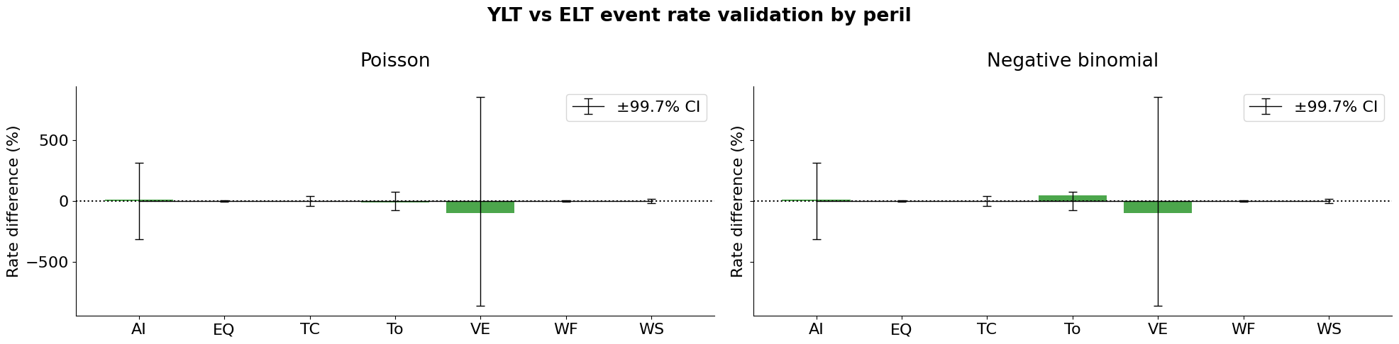
The first step is to transform the Event Loss Table (ELT; introduced in Tutorial 2) into a standard Year Loss Table (YLT), which explicitly represents the sequence of events occurring within each simulated year. This transformation is performed using the gen_YLT() function. The term standard is used to distinguish a YLT derived directly from an ELT from the more sophisticated approaches described in Section 2, where events may interact with one another and with the environment.

For each peril, an event count distribution must be specified. By default, event counts are assumed to follow a Poisson distribution, representing independent event occurrences. Alternatively, a negative binomial distribution can be used to model event clustering, as is observed for example for tropical cyclones (TC).

As the number of simulated years (Nsim) increases, the Average Annual Loss (AAL) estimated from the YLT should converge to the AAL obtained from the ELT for both count distributions. This is because the negative binomial distribution preserves the expected annual event count, while allowing for greater variability in the number of events per year.

Nsim = int(1e5)            # number of year-simulations, user-defined


AAL_ELT = np.sum(ELT['lbd'] * ELT['loss']) * 1e-6

## 1. Standard Poisson sampling
countDistr = {peril: 'Poisson' for peril in perils}
YLT_poi = GenMR_dyn.gen_YLT(ELT, Nsim, countDistr)
AAL_YLT_poi = np.sum(YLT_poi['loss']) / Nsim * 1e-6

annual_loss_poi = YLT_poi.groupby('simID')['loss'].sum().reindex(np.arange(1, Nsim+1), fill_value=0) # fill gaps
SE_poi = annual_loss_poi.std() / np.sqrt(Nsim) * 1e-6

print(f'AAL ELT (M. $): {AAL_ELT:.2f}')
print('** POISSON **')
print(f'AAL YLT Poisson (M. $): {AAL_YLT_poi:.3f} ± {3*SE_poi:.2f}  (99.7% CI)')
print(f'Within tolerance: {abs(AAL_ELT - AAL_YLT_poi) <= 3 * SE_poi}')

## 2. Incl. peril-based clustering option
countDistr = {peril: 'Poisson' for peril in perils}
countDistr['TC'] = 'negative binomial'             # clustering for specified perils

# overdispersion parameter: phi = var/lbd - 1 
clustering_phi = {
    'TC': .91                                      # from Mignan (2025, CUP textbook)
}

YLT_nb = GenMR_dyn.gen_YLT(ELT, Nsim, countDistr, clustering_phi)
AAL_YLT_nb = np.sum(YLT_nb['loss']) / Nsim * 1e-6

annual_loss_nb = YLT_nb.groupby('simID')['loss'].sum().reindex(np.arange(1, Nsim+1), fill_value=0)
SE_nb = annual_loss_nb.std() / np.sqrt(Nsim) * 1e-6
print('** NEGATIVE BINOMIAL (for selected perils) **')
print(f'AAL YLT nb (M. $): {AAL_YLT_nb:.3f} ± {3*SE_nb:.3f}  (99.7% CI)')
print(f'Within tolerance: {abs(AAL_ELT - AAL_YLT_nb) <= 3*SE_nb}')

AAL ELT (M. $): 759.92
** POISSON **
AAL YLT Poisson (M. $): 780.552 ± 57.35  (99.7% CI)
Within tolerance: True
** NEGATIVE BINOMIAL (for selected perils) **
AAL YLT nb (M. $): 744.365 ± 55.677  (99.7% CI)
Within tolerance: True

def validation_sim_rates(ELT, YLT, Nsim, label, ax, phi_dict = None):
    perils = ELT['ID'].unique()
    diff = []
    tol  = []
    for peril in perils:
        indperil = ELT['ID'] == peril
        lbd = ELT.loc[indperil, 'lbd'].sum()
        rate_YLT = YLT[YLT['evID'].isin(ELT.loc[indperil, 'evID'])].shape[0] / Nsim
        diff.append((rate_YLT - lbd) / lbd * 100)

        phi = phi_dict[peril] if (phi_dict and peril in phi_dict) else 0.
        tol.append(3 * np.sqrt(lbd * (1 + phi) / Nsim) / lbd * 100)          # 3 * SE

    colors = ['tomato' if abs(d) > t else 'green' for d, t in zip(diff, tol)]
    ax.bar(perils, diff, color=colors, alpha = .7)
    ax.errorbar(perils, [0] * len(perils), yerr = tol, color = 'black', capsize=4, lw=1, label='±99.7% CI')
    ax.axhline(0, color='black', linestyle = 'dotted')
    ax.set_ylabel('Rate difference (%)')
    ax.set_title(label, pad = 20)
    ax.spines['right'].set_visible(False)
    ax.spines['top'].set_visible(False)
    ax.legend()


plt.rcParams['font.size'] = '16'
fig, ax = plt.subplots(1, 2, figsize=(20, 5), sharey = True)
validation_sim_rates(ELT, YLT_poi, Nsim, 'Poisson', ax[0])
validation_sim_rates(ELT, YLT_nb,  Nsim, 'Negative binomial',  ax[1])
fig.suptitle('YLT vs ELT event rate validation by peril', fontweight='bold')
plt.tight_layout();

1.2. Time occurrence implementation

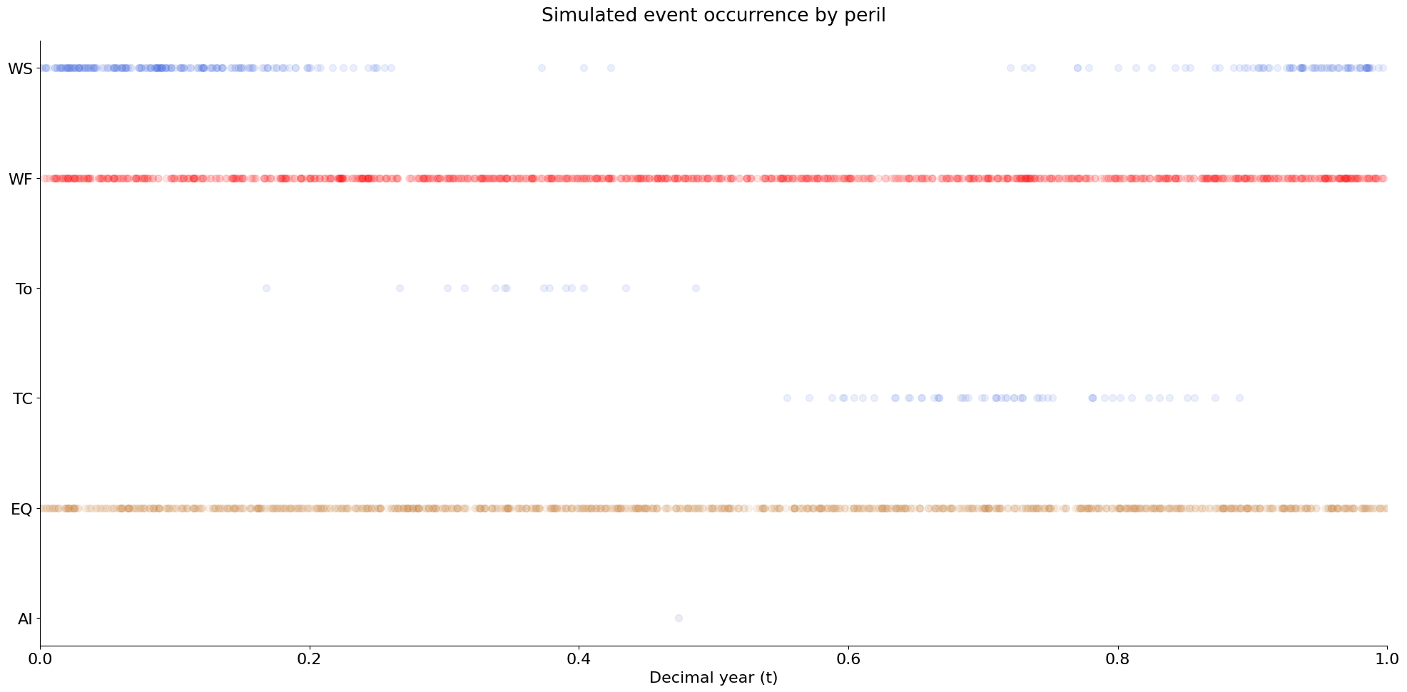
In dynamic catastrophe risk modelling, each simulated event must be assigned an occurrence time. This is specified by the variable t in the YLT and expressed as a decimal year in the interval (0, 1). Before introducing physically based compound-event modelling (Section 2), event occurrence times can be sampled either from a uniform distribution or from a von Mises distribution using sample_seasonal_t(). The von Mises distribution provides a phenomenological representation of seasonality based on empirical observations, and is intended here for meteorological perils (Li, TC, To, WS). In contrast, Section 2.1 introduces seasonality that emerges from explicit physical constraints, enabling the modelling of climatic perils.

####################################
## Seasonal meteorological perils ##
####################################

# consider only one YLT: poisson or incl. negative binomial for illustration
YLT = YLT_poi.copy()
YLT['ID'] = YLT['evID'].str[:2]

year = 0     # could be the current or next year, e.g., 2027 - only cosmetic at this stage
             # (see long-term trend section for year relevance)


    
## random uniform time (default) ##
YLT['t'] = year + np.random.uniform(0, 1, size = len(YLT))   # some to be overwritten below
YLT = YLT[['simID', 'evID', 'ID', 't', 'S', 'loss']]



## seasonal (for meteorological perils) ##
seasonal_par = {
    'WS': {'peak_day': 15,  'kappa': 3},   # mid-January
    'To': {'peak_day': 130, 'kappa': 5},   # early May, narrower season
    'Li': {'peak_day': 130, 'kappa': 5},   # same as Li since CS -> (To, Li), see Tutorial 2
    'TC': {'peak_day': 260, 'kappa': 4},   # mid-September
}

for ID, par in seasonal_par.items():
    ind = YLT['ID'] == ID
    n = ind.sum()
    if n == 0:
        continue
    YLT.loc[ind, 't'] = GenMR_dyn.sample_seasonal_t(par['peak_day'], par['kappa'], n)
    
    
# time series plot
fig, ax = plt.subplots(figsize=(20, 10))

perils = np.sort(YLT['ID'].unique())
colors = {p: GenMR_utils.col_peril(p) for p in perils}

nmax = 1000
for i, ID in enumerate(perils):
    subset = YLT[YLT['ID'] == ID]
    n = np.min([len(subset),nmax])
    ax.scatter(subset['t'].values[:nmax], np.full(n, i),
               color = colors[ID], alpha = .1, s = 50, label = ID)

ax.set_yticks(range(len(perils)))
ax.set_yticklabels(perils)
ax.set_xlabel('Decimal year (t)')
ax.set_xlim(0, 1)
ax.spines['right'].set_visible(False)
ax.spines['top'].set_visible(False)
ax.set_title('Simulated event occurrence by peril', pad = 20)
plt.tight_layout();

2. Compound event modelling

ONGOING DEVELOPMENT…

A compound event is defined as an extreme event resulting from the interplay of multiple physical processes. It encompasses various forms of interconnected phenomena, including simple one-to-one chains of events (i.e., domino effects), external forcing factors simultaneously affecting multiple perils, combinations of events triggering subsequent events, feedback loops, and more complex scenarios that integrate all of these mechanisms.

Fig. 1. Concept of Compound Event. (a) Combinations of causally unrelated events: Known as the “Perfect Storm” concept, this refers to simultaneous events in the same region, such as an earthquake and a storm. (b) Simple one-to-one chains of events: Examples include successive explosions, fires, and toxic spills at critical infrastructures. (c) Common external forcing factor: A shared external influence, such as warming, alters the probability or intensity of multiple events—for instance, droughts, heatwaves, and wildfires. (d) System feedback loops: Feedback mechanisms that reinforce events, such as the escalation of an epidemic into a pandemic. Compound events may also involve intricate combinations of all the above factors.

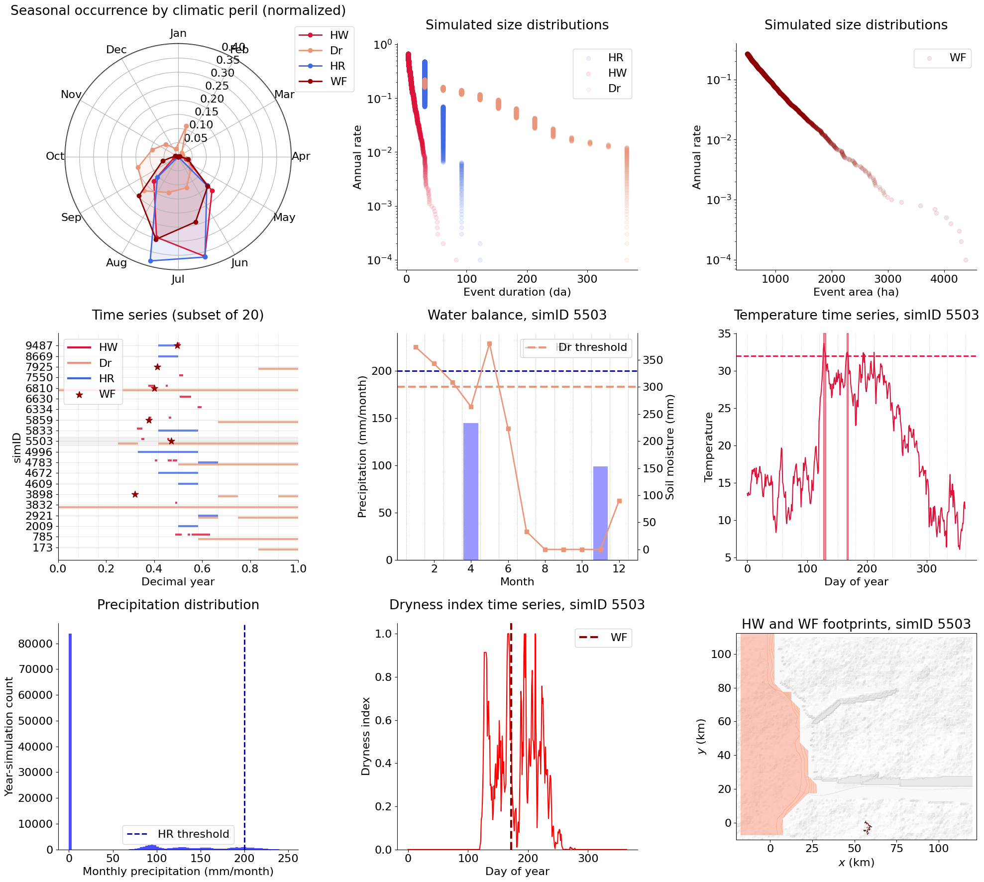
Section 2.1 first considers temperature as a common external forcing influencing the climatic perils HW, Dr, and WF (incl. anticorrelated heavy rain episodes HR). This framework naturally produces physically based seasonality and a concentration of extreme events during stochastic temperature anomalies. It also provides a direct pathway for incorporating the effects of global warming, which will be explored in the future Section 3.

Section 2.2 will introduce one-to-one event chains and cascading events. UNDER CONSTRUCTION.

Note that coincident events (i.e., perfect storms) are already represented through the event-time sampling introduced in Section 1.2.

At this stage, the focus is on the dynamics of event occurrence through the Year Event Table (YET), independently of the Year Loss Table (YLT). This separation allows the physical mechanisms governing compound events to be developed before extending the framework to loss assessment. The integration of losses will be addressed in the future Section 3.

2.1. Common environmental drivers

2.1.1. Temperature (& water content) as external forcing factor

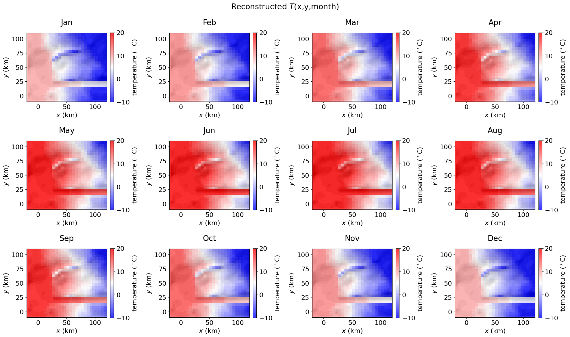
Intra-annual temperature variations are simulated using the Energy Balance Climate Model (EBCM) introduced in Tutorial 1 on environmental layers. The same EBCM framework was also used in Tutorial 2 to demonstrate the emergence of heatwaves (HW) and droughts (Dr).

Primary heavy rainfall (HR) events, introduced ad hoc in Tutorial 2, are now modelled explicitly to illustrate their relationship with heatwaves, droughts, and wildfires through alternating atmospheric circulation regimes.

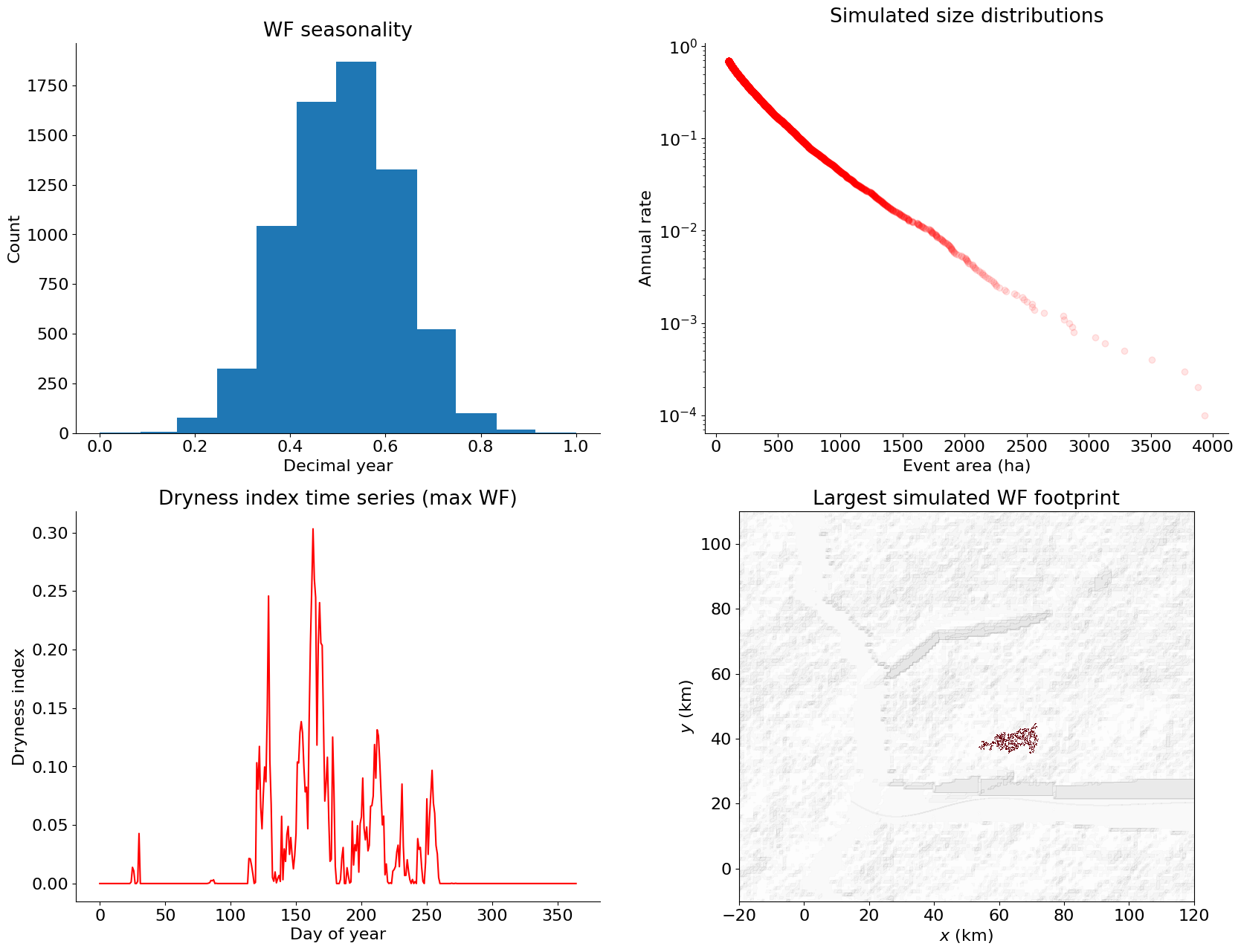
Wildfire (WF) occurrence times are here defined by introducing a dryness index, which combines the effects of high temperature and lack of soil moisture, hence relating WF to HW, Dr (correlated) and HR (anti-correlated).

The hazard models of Tutorial 2 are only slightly modified and here implemented in gen_YET_*() functions to simulate climatic event time series.

Note: Additional HR events triggered by individual storms may be incorporated later in Section 2.2. The term heavy rainfall is used instead of rainstorm because HR is represented here as a prolonged, month-scale climatological water forcing rather than as an individual multi-day storm event. Such storm-related rainfall events will be considered separately, as rainfall components associated with windstorms (WS) or tropical cyclones (TC).

## EBCM seasonal driver (climatical & meteorological perils) ##
days_per_mon = GenMR_utils.days_per_mon
ndays = sum(GenMR_utils.days_per_mon)  # 365
moni_da = np.array([m + .5 + d / days_per_mon[m] for m, nday in enumerate(days_per_mon) for d in range(nday)])
            # t = (mon - .5)/12 in calc_T0_EBCM()

# atmoLayer.T not used, instead: from month to day resolution & spatial footprint downscaled for fast computation
f = 50
grid_downscaled = GenMR_env.downscale_RasterGrid(grid, f, appl = 'pooling')
topoLayer_downscaled = copy.deepcopy(topoLayer)
topoLayer_downscaled.grid = grid_downscaled
topoLayer_downscaled.z = GenMR_utils.pooling(topoLayer.z, f, method = 'mean')


T0, _, _ = GenMR_env.EnvLayer_atmo.calc_T0_EBCM(grid.lat_deg, moni_da)
topo_z_corr = topoLayer_downscaled.z.copy() * 1e-3       # m to km
topo_z_corr[topo_z_corr < 0.] = 0                        # water surface at z=0
T = GenMR_env.EnvLayer_atmo.calc_T_z(topo_z_corr[None, :, :], T0[:, None, None], \
                                     lapse_rate = atmoLayer.par['lapse_rate_degC/km'])

# plot mean monthly T
month_names = ['Jan','Feb','Mar','Apr','May','Jun','Jul','Aug','Sep','Oct','Nov','Dec']
day_bounds = np.concatenate([[0], np.cumsum(days_per_mon)])  # cum. day boundaries, length 13

plt.rcParams['font.size'] = '16'
fig, axes = plt.subplots(3, 4, figsize=(20, 12))
axes = axes.ravel()

for ax, month in zip(axes, range(1, 13)):
    start, end = day_bounds[month - 1], day_bounds[month]
    T_mon = T[start:end].mean(axis=0)

    ax.contourf(grid_downscaled.xx, grid_downscaled.yy, GenMR_env.ls.hillshade(topoLayer_downscaled.z, \
                                                            vert_exag=.1), cmap='gray')
    imgT = ax.pcolormesh(grid_downscaled.xx, grid_downscaled.yy, T_mon, cmap = 'bwr', \
                         vmin=-10, vmax=20, alpha = .8)
    ax.set_title(month_names[month - 1], pad = 20)
    ax.set_xlabel('$x$ (km)')
    ax.set_ylabel('$y$ (km)')
    ax.set_xlim(xmin, xmax)
    ax.set_ylim(ymin, ymax)
    ax.set_aspect(1)
    fig.colorbar(imgT, ax = ax, fraction = .04, pad = .04, label = 'temperature ($^\circ$C)')

plt.suptitle(r'Reconstructed $T$(x,y,month)')
plt.tight_layout();

##############################
## Seasonal climatic perils ##
##############################

Nsim = int(1e4)            # number of year-simulations, user-defined



# shared delta-temperature time series for HW, Dr and HR
Ndays = T.shape[0]
DT_peryr, DT_adv_month, DT_adv_daily = GenMR_dyn.sample_DT_stoch(src.par['HW'], Nsim, Ndays)

# NB: the following peril parameters are selected so that all size (duration)-distributions are reasonably close
# for illustration purposes. In a generic context, there is no clear constraint on these values.
print('HW modelling')
src.par['HW']['T_th'] = 32             # Minimum temperature threshold (°C)
YET_HW, catalog_hazFp_HW, T_sav_daily_stoch = \
    GenMR_dyn.gen_YET_HW(T0, T, src.par['HW'], DT_peryr, DT_adv_daily, Nsim)

print('Dr/HR modelling')
src.par['Dr']['hw_th'] = .1            # %tage of normal soil water content hw_fc_m to be declated Dr
src.par['Dr']['Dr_stress_mean'] = .5   # mean fraction of hw_fc depleted before year starts
src.par['Dr']['Dr_stress_k'] = 4.      # Beta concentration: higher = tighter around the mean
Dr_stress = GenMR_dyn.sample_Dr_stress(src.par['Dr'], Nsim)

src.par['Dr']['HR_th'] = 200           # mm/month

#atmoLayer.par['vz_subs_asc'] = [-.001, .02]
atmoLayer.par['vz_subs_asc'] = [-.001, .01]    # reduce amount of rain - needs calibration

moni = np.arange(12)+1
T0_mo, _, _ = GenMR_env.EnvLayer_atmo.calc_T0_EBCM(src.par['Dr']['lat_deg'], moni)
YET_Dr, YET_HR, S_t_saved, I_rain_saved = GenMR_dyn.gen_YET_Dr_HR(T0_mo, src.par['Dr'], atmoLayer.par, \
                                          soilLayer.par, DT_peryr, DT_adv_month, Dr_stress, Nsim)


print('WF modelling')
src.par['WF']['ratio_grass'] = .45    # reduced compared to Tutorial 2 since no long-term tree regrowth
src.par['WF']['lbd0'] = .3            # rate calibration given dryness level
src.par['WF']['n_dryness'] = 3.       # concentration factor (narrowing occurrence month range)
                                      # WARNING: increasing n reduces likelihood of WF, correct by increasing lbd0
src.par['WF']['Tmin'] = 20.           # min temperature above which pr(burn) non-zero (for dryness index)
src.par['WF']['Smin_ha'] = 500


## define dryness index (compound effect)
S_t_daily = np.repeat(S_t_saved, GenMR_utils.days_per_mon, axis = 1)
hw_fc = soilLayer.par['hw_fc_m'] * 1e3
Dr_th = hw_fc * src.par['Dr']['hw_th']
Snorm_t = 1. - np.clip((S_t_daily - Dr_th) / (hw_fc - Dr_th), 0, 1)
Tnorm_t = np.clip((T_sav_daily_stoch-src.par['WF']['Tmin']) / (src.par['HW']['T_th']-src.par['WF']['Tmin']), 0, 1)
D_t = (Tnorm_t * Snorm_t) ** src.par['WF']['n_dryness']  # n>1 sharpens sensitivity (à la FFDI/KBDI curing curves)

#I_rain_daily = np.repeat(I_rain_saved, GenMR_utils.days_per_mon, axis = 1)  # to be explored if S_t not enough
#D_t[I_rain_daily > 0.] = 0

YET_WF, catalog_hazFp_WF = GenMR_dyn.gen_YET_WF(src, urbLandLayer, D_t)

HW modelling
Dr/HR modelling
WF modelling
10000/10000

## plots ##
n_sample = 20        # number of plotted time series (simulation years)
seed = 2             # for time series sampling - decide from figure below
sample_ID = 10       # which one of the sampled time series to explore (index) - choose from figure below

np.random.seed(seed)
all_simIDs = np.unique(np.concatenate([
    YET_HW['simID'].values, YET_Dr['simID'].values, YET_HR['simID'].values]))
sample = np.random.choice(all_simIDs, size = min(n_sample, len(all_simIDs)), replace = False)
sample.sort()


plt.rcParams['font.size'] = '16'
fig, ax = plt.subplots(3,3, figsize=(20, 18))

gs = ax[0,0].get_gridspec()
ax[0,0].remove()
ax00 = fig.add_subplot(gs[0,0], projection='polar')
ax00.set_theta_zero_location('N')
ax00.set_theta_direction(-1)

bins = np.linspace(0, 2*np.pi, 13)  # 12 monthly bins around circle
width = 2 * np.pi / 12
for df, color, label in [(YET_HW, GenMR_utils.col_peril('HW'), 'HW'),
                         (YET_Dr, GenMR_utils.col_peril('Dr'), 'Dr'),
                         (YET_HR, GenMR_utils.col_peril('HR'), 'HR'),
                         (YET_WF, 'darkred', 'WF')]:
    if df.empty:
        continue
    theta = df['t'].values * 2*np.pi
    counts, _ = np.histogram(theta, bins=bins)
    counts = counts / counts.sum()             # normalized
    centers = (bins[:-1] + bins[1:]) / 2
    ax00.plot(np.append(centers, centers[0]), np.append(counts, counts[0]),
            color=color, marker='o', label=label, lw=2)
    ax00.fill(np.append(centers, centers[0]), np.append(counts, counts[0]),
            color=color, alpha=.1)

ax00.set_xticks(np.linspace(0, 2*np.pi, 12, endpoint=False))
ax00.set_xticklabels(GenMR_utils.month_labels_short)
ax00.set_title('Seasonal occurrence by climatic peril (normalized)', pad = 20)
ax00.legend(loc='upper right', bbox_to_anchor=(1.3, 1.1))


## event size distributions ##
S_HW, Sdistr_HW = GenMR_utils.calc_Sdistr_empirical(YET_HW, 'S')
S_Dr, Sdistr_Dr = GenMR_utils.calc_Sdistr_empirical(YET_Dr, 'S')
S_HR, Sdistr_HR = GenMR_utils.calc_Sdistr_empirical(YET_HR, 'S')

ax[0,1].scatter(S_HR /12*Ndays, Sdistr_HR, color = GenMR_utils.col_peril('HR'), alpha = .1, label ='HR')
ax[0,1].scatter(S_HW, Sdistr_HW, color = GenMR_utils.col_peril('HW'), alpha = .1, label ='HW')
ax[0,1].scatter(S_Dr /12*Ndays, Sdistr_Dr, color = GenMR_utils.col_peril('Dr'), alpha = .1, label ='Dr')
ax[0,1].set_yscale('log')
ax[0,1].set_xlabel('Event duration (da)')
ax[0,1].set_ylabel('Annual rate')
ax[0,1].set_title('Simulated size distributions', pad = 20)
ax[0,1].spines['right'].set_visible(False)
ax[0,1].spines['top'].set_visible(False)
ax[0,1].legend()

S_WF, Sdistr_WF = GenMR_utils.calc_Sdistr_empirical(YET_WF, 'S')

ax[0,2].scatter(S_WF, Sdistr_WF, color = 'darkred', alpha = .1, label ='WF')
ax[0,2].set_yscale('log')
ax[0,2].set_xlabel('Event area (ha)')
ax[0,2].set_ylabel('Annual rate')
ax[0,2].set_title('Simulated size distributions', pad = 20)
ax[0,2].spines['right'].set_visible(False)
ax[0,2].spines['top'].set_visible(False)
ax[0,2].legend()


## sampled time series ##
for r in range(len(sample)):
    ax[1,0].axhline(r, color='gray', lw=.5, alpha=.3, zorder=0)

ax[1,0].axhspan(sample_ID - .4, sample_ID + .4, color='grey', alpha = .1, zorder = 0)

for df, color, label, dur_norm, plt_shift in [(YET_HW, GenMR_utils.col_peril('HW'), 'HW', Ndays, .2),
                                       (YET_Dr, GenMR_utils.col_peril('Dr'), 'Dr', 12, -.2),
                                       (YET_HR, GenMR_utils.col_peril('HR'), 'HR', 12, 0.)]:
    sub = df[df['simID'].isin(sample)]
    row = np.searchsorted(sample, sub['simID'].values)
    t_start = sub['t'].values
    t_end = t_start + sub['S'].values / dur_norm

    for r, t0, t1 in zip(row, t_start, t_end):
        ax[1,0].plot([t0, t1], [r + plt_shift, r + plt_shift], color=color, lw=3, solid_capstyle='butt', \
                     alpha=.8, zorder=2)
    ax[1,0].plot([], [], color=color, lw=3, label=label)

sub_WF = YET_WF[YET_WF['simID'].isin(sample)]
row = np.searchsorted(sample, sub_WF['simID'].values)
ax[1,0].scatter(sub_WF['t'], row, color = 'darkred', marker = '*', s = 100, label = 'WF', zorder=3)

for m in range(1, 12):
    ax[1,0].axvline(m/12, color='grey', lw=.5, ls=':', alpha=.5, zorder=0)

ax[1,0].set_yticks(range(len(sample)))
ax[1,0].set_yticklabels(sample)
ax[1,0].set_xlabel('Decimal year')
ax[1,0].set_ylabel('simID')
ax[1,0].set_xlim(0, 1)
ax[1,0].spines['right'].set_visible(False)
ax[1,0].spines['top'].set_visible(False)
ax[1,0].legend()
ax[1,0].set_title(f'Time series (subset of {n_sample})', pad = 20)


## Dr/HR process visualisation ##
sim = sample[sample_ID] - 1

Dr_th = soilLayer.par['hw_fc_m'] * 1e3 * src.par['Dr']['hw_th']
I_rain_mo = I_rain_saved[sim,:]
S_t = S_t_saved[sim,:]

months = np.arange(1, 13)
ax[1,1].bar(months, I_rain_mo, alpha=.4, color='blue')
ax[1,1].axhline(src.par['Dr']['HR_th'], color='darkblue', ls='dashed', lw = 2, label='HR threshold')
ax[1,1].set_xlabel('Month')
ax[1,1].set_ylabel('Precipitation (mm/month)')
ax[1,1].set_ylim(0, 1.2 * np.max([np.max(I_rain_mo), src.par['Dr']['HR_th']]))
ax[1,1].spines['right'].set_visible(False)
ax[1,1].spines['top'].set_visible(False)
ax[1,1].legend()

ax2 = ax[1,1].twinx()
ax2.plot(months, S_t, color = GenMR_utils.col_peril('Dr'), marker = 's', linewidth = 2)
ax2.axhline(Dr_th, color = GenMR_utils.col_peril('Dr'), linestyle = 'dashed', lw = 3, label = 'Dr threshold')
ax2.set_ylabel('Soil moisture (mm)')
ax2.spines['top'].set_visible(False)
ax2.legend()

ax[1,1].set_title(f'Water balance, simID {sim+1}', pad = 20)
for m in range(0, 13):
    ax[1,1].axvline(m + .5, color='grey', lw=.5, ls=':', alpha=1, zorder=0)


## ZOOMING IN ONE SPECIFIED TIME SERIES
sim = sample[sample_ID] - 1
HWev = YET_HW[YET_HW['simID'] == sim + 1]
WFev = YET_WF[YET_WF['simID'] == sim + 1]


## stochastic temperature time series ##
ax[1,2].plot(np.arange(Ndays), T_sav_daily_stoch[sim,:], color = GenMR_utils.col_peril('HW'))
month_starts = np.concatenate(([0], np.cumsum(GenMR_utils.days_per_mon)))
for d in month_starts:
    ax[1,2].axvline(d, color='grey', lw=.5, ls='dotted', alpha=.5, zorder=0)
for i in range(len(HWev)):
    ax[1,2].axvspan(HWev['t'].values[i] * 365, HWev['t'].values[i] * 365 + HWev['S'].values[i], \
                color = GenMR_utils.col_peril('HW'), alpha=.5)
ax[1,2].axhline(src.par['HW']['T_th'], color=GenMR_utils.col_peril('HW'), ls='dashed', lw = 2, \
                label='HW threshold')
ax[1,2].set_xlabel('Day of year')
ax[1,2].set_ylabel('Temperature')
ax[1,2].spines['right'].set_visible(False)
ax[1,2].spines['top'].set_visible(False)
ax[1,2].set_title(f'Temperature time series, simID {sim+1}', pad = 20)


## precipitation distributrion (HR) ##
ax[2,0].hist(I_rain_saved.flatten(), bins=80, color='blue', alpha=.7)
#for q in [50, 90, 95, 99]:
#    val = np.percentile(I_rain_saved.flatten(), q)
#    print(f'p{q}: {val:.1f} mm/month')
ax[2,0].axvline(src.par['Dr']['HR_th'], color='darkblue', ls='dashed', lw = 2, label='HR threshold')
ax[2,0].set_xlabel('Monthly precipitation (mm/month)')
ax[2,0].set_ylabel('Year-simulation count')
ax[2,0].set_title('Precipitation distribution', pad = 20)
ax[2,0].legend()
ax[2,0].spines['right'].set_visible(False)
ax[2,0].spines['top'].set_visible(False)


## dryness index (WF) ##
ax[2,1].plot(np.arange(365), D_t[sim,:], color = 'red')
for i in range(len(WFev)):
    ax[2,1].axvline(WFev['t'].values[i] * 365, color = 'darkred', linestyle = 'dashed', \
                    label='WF' if i == 0 else None, lw = 3)
ax[2,1].set_xlabel('Day of year')
ax[2,1].set_ylabel('Dryness index')
ax[2,1].set_ylim(0,1.05)
ax[2,1].set_title(f'Dryness index time series, simID {sim+1}', pad = 20)
ax[2,1].spines['right'].set_visible(False)
ax[2,1].spines['top'].set_visible(False)
ax[2,1].legend()


## footprints (HW + WF) ## - HR and Dr are constant in space (Digital Template small enough)
ax[2,2].contourf(grid.xx, grid.yy, GenMR_env.ls.hillshade(topoLayer.z, vert_exag=.1), cmap='gray', alpha = .1)

if len(HWev) != 0:
    HWid_max = HWev[HWev['S'] == np.max(HWev['S'])]['evID'].values[0]
    ax[2,2].contourf(grid_downscaled.xx, grid_downscaled.yy, catalog_hazFp_HW[HWid_max], cmap = 'Reds', \
                alpha = .5, vmin=30, vmax = 40)

for i in range(len(WFev)):
    WF_fp_max = np.full(grid.xx.shape, np.nan)
    WFid_i = WFev['evID'].values[i]
    WF_fp_max[catalog_hazFp_WF[WFid_i]] = 1
    ax[2,2].pcolormesh(grid.xx, grid.yy, WF_fp_max, cmap = 'Reds', alpha = 1, vmin=0, vmax = 1)

ax[2,2].set_xlabel('$x$ (km)')
ax[2,2].set_ylabel('$y$ (km)')
ax[2,2].set_title(f'HW and WF footprints, simID {sim+1}')
ax[2,2].set_aspect(1)

plt.tight_layout();

# add HW, Dr and HR to original YLT

#for YET in [YET_HW, YET_Dr, YET_HR]:
#    YET['loss'] = np.nan

#YLT = pd.concat([YLT, YET_HW, YET_Dr, YET_HR], ignore_index=True)
#YLT = YLT.sort_values(['simID', 't']).reset_index(drop=True)

## WILDFIRE CASE ## - modified version for probabilistic fire propagation instead of deterministic

## FOR TESTING ... 



import os
from skimage import measure



def sample_WF_t(D_t_1sim, lbd0):
    '''
    D_t_1sim : daily dryness index for one simulated year (0-1), shape (Ndays,)
    lbd0 : calibrated scale so that lambda(t) = lbd0 * D_t is a daily ignition rate
    '''
    lbd_t = lbd0 * D_t_1sim
    lbd_max = lbd_t.max()
    if lbd_max <= 0:
        return np.array([], dtype=int)

    Ndays = len(D_t_1sim)
    # homogeneous proposal process at rate lbd_max
    n_candidates = np.random.poisson(lbd_max * Ndays)
    candidate_days = np.random.randint(0, Ndays, size=n_candidates)

    # thinning step
    accept_prob = lbd_t[candidate_days] / lbd_max
    accept = np.random.random(n_candidates) < accept_prob
    occurrence_days = np.sort(candidate_days[accept])
    return occurrence_days

def percolate_cluster(seed_idx, p_edge_grid):
    '''
    NOT YET FULLY TESTED - so far not used
    '''
    ny, nx = p_edge_grid.shape
    visited = np.zeros_like(p_edge_grid, dtype=bool)
    sy, sx = np.unravel_index(seed_idx, p_edge_grid.shape)
    stack = [(sy, sx)]
    visited[sy, sx] = True
    while stack:
        y, x = stack.pop()
        for dy, dx in ((1,0), (-1,0), (0,1), (0,-1)):
            ny_, nx_ = y+dy, x+dx
            if 0 <= ny_ < ny and 0 <= nx_ < nx and not visited[ny_, nx_] and S[ny_, nx_] == 1:
                if np.random.random() < p_edge_grid[ny_, nx_]:
                    visited[ny_, nx_] = True
                    stack.append((ny_, nx_))
    return visited

def gen_YET_WF(src, urbLandLayer, D_t, method = 'deterministic'):
    '''
    '''
    Nsim = D_t.shape[0]    # use same number as HW and Dr
    landuse_S = copy.copy(urbLandLayer.S)

    # Fuel includes forest (S=1), later updated with wood building
    FuelClass = [1]

    # only used if method = 'probabilistic' (to move to env. layer):
    FuelCoef_by_class = {
                -1: 0.,   # water
                0: 0.,    # grassland
                1: 1.,    # forest
                2: 0.,    # urban - residential
                3: 0.,    # urban - industrial
                4: 0.,    # urban - commercial
                5: .6,    # wheat
                6: .6,    # maize
    }
    FuelCoef = np.vectorize(FuelCoef_by_class.get)(landuse_S)
    

    YET_WF_list = []
    catalog_hazFp_WF = {}
    evID_counter = 0
    for sim in range(Nsim):
        # stochastic fuel to grass distribution
        indFuel = np.where(np.isin(landuse_S.flatten(), FuelClass))[0]
        indFuel2Grass = np.random.choice(indFuel, size = int(len(indFuel) * src.par['WF']['ratio_grass']),
                        replace = False)    
        landuse_S4WF_flat = landuse_S.flatten()
        landuse_S4WF_flat[indFuel2Grass] = 0                           # grassland
        indFuel = np.where(np.isin(landuse_S4WF_flat, FuelClass))[0]   # updated
        # add wood buildings to fuel state:
        indwoodBldg = np.where(urbLandLayer.bldg_type.flatten() == 'W')[0]
        landuse_S4WF_flat[indwoodBldg] = 1                             # forest-like
        landuse_S4WF0 = landuse_S4WF_flat.reshape(landuse_S.shape)
        # connectivity
        indconnect = np.where(np.isin(landuse_S4WF_flat, FuelClass))[0]
        grid_connect_flat = np.zeros_like(landuse_S4WF_flat)
        grid_connect_flat[indconnect] = 1
        grid_connect0 = grid_connect_flat.reshape(landuse_S.shape)
        
        # can be updated within a year
        grid_connect = grid_connect0.copy()
        landuse_S4WF = landuse_S4WF0.copy()
        
        simID = sim + 1
        if simID % 1000 == 0:
            print(f'{simID}/{Nsim}', end='\r', flush=True)

        WF_days = sample_WF_t(D_t[sim, :], src.par['WF']['lbd0'])

        for ev_i in range(len(WF_days)):
            ignition_xy = np.random.choice(indFuel)
            fp_WF = np.full(grid_connect.shape, np.nan)

            if grid_connect.flat[ignition_xy] == 1:
                if method == 'deterministic':
                    S_clumps = measure.label(grid_connect, connectivity = 1)
                    clump_WF = S_clumps.flatten()[ignition_xy]
                    indWF = S_clumps == clump_WF
                elif method == 'probabilistic':
                    pmax = .5   # critical regime
                    p_edge = pmax * D_t[sim, WF_days[ev_i]] * FuelCoef
                    indWF = percolate_cluster(ignition_xy[0], p_edge)
                
                fp_WF[indWF] = 1
                grid_connect[indWF] = 0
                landuse_S4WF[indWF] = 0

                burntArea_cells = np.sum(fp_WF == 1)
                area_ha = burntArea_cells * (urbLandLayer.grid.w ** 2) * 100

                #burntBldgBlocks_cells = np.sum(indWF.flatten()[indwoodBldg])   # to use later for loss calc...

                if area_ha >= src.par['WF']['Smin_ha']:
                    evID_counter += 1
                    evID = f'WF{evID_counter}'
                    
                    catalog_hazFp_WF[evID] = indWF   #fp_WF

                    t = WF_days[ev_i] / 365.
                    YET_WF_list.append({'simID': simID, 'evID': evID, 'ID': 'WF', 't': t, 'S': area_ha})


    return pd.DataFrame(YET_WF_list), catalog_hazFp_WF
          
            
            

        
# change WF parameterisation for new model testing
src.par['WF']['ratio_grass'] = .45    # reduced compared to Tutorial 2 since no long-term tree regrowth

src.par['WF']['lbd0'] = .1            # rate calibration
src.par['WF']['n_dryness'] = 2.       # concentration factor
src.par['WF']['Tmin'] = 20.           # min temperature above which pr(burn) non-zero

src.par['WF']['Smin_ha'] = 100


## define dryness index (compound effect)
S_t_daily = np.repeat(S_t_saved, GenMR_utils.days_per_mon, axis = 1)
hw_fc = soilLayer.par['hw_fc_m'] * 1e3
Dr_th = hw_fc * src.par['Dr']['hw_th']
Snorm_t = 1. - np.clip((S_t_daily - Dr_th) / (hw_fc - Dr_th), 0, 1)
Tnorm_t = np.clip((T_sav_daily_stoch-src.par['WF']['Tmin']) / (src.par['HW']['T_th']-src.par['WF']['Tmin']), 0, 1)

D_t = (Tnorm_t * Snorm_t) ** src.par['WF']['n_dryness']  # n>1 sharpens sensitivity (à la FFDI/KBDI curing curves)



YET_WF, catalog_hazFp_WF = gen_YET_WF(src, urbLandLayer, D_t, method = 'deterministic')

10000/10000

plt.rcParams['font.size'] = '16'
fig, ax = plt.subplots(2,2, figsize=(20, 15))

bins_da = np.concatenate(([0], np.cumsum(GenMR_utils.days_per_mon)))
ax[0,0].hist(YET_WF['t'], bins = bins_da / 365.)
ax[0,0].set_xlabel('Decimal year')
ax[0,0].set_ylabel('Count')
ax[0,0].set_title('WF seasonality')
ax[0,0].spines['right'].set_visible(False)
ax[0,0].spines['top'].set_visible(False)

WFid_max = YET_WF[YET_WF['S'] == np.max(YET_WF['S'])]['evID'].values[0]
simID_max = YET_WF[YET_WF['S'] == np.max(YET_WF['S'])]['simID'].values[0]

ax[1,0].plot(np.arange(365), D_t[simID_max-1,:], color = 'red')
ax[1,0].set_xlabel('Day of year')
ax[1,0].set_ylabel('Dryness index')
ax[1,0].set_title('Dryness index time series (max WF)')
ax[1,0].spines['right'].set_visible(False)
ax[1,0].spines['top'].set_visible(False)

S_WF, Sdistr_WF = GenMR_utils.calc_Sdistr_empirical(YET_WF, 'S')

ax[0,1].scatter(S_WF, Sdistr_WF, color = GenMR_utils.col_peril('WF'), alpha = .1)
ax[0,1].set_yscale('log')
ax[0,1].set_xlabel('Event area (ha)')
ax[0,1].set_ylabel('Annual rate')
ax[0,1].set_title('Simulated size distributions', pad = 20)
ax[0,1].spines['right'].set_visible(False)
ax[0,1].spines['top'].set_visible(False)

WF_fp_max = np.full(grid.xx.shape, np.nan)
WF_fp_max[catalog_hazFp_WF[WFid_max]] = 1

ax[1,1].contourf(grid.xx, grid.yy, GenMR_env.ls.hillshade(topoLayer.z, vert_exag=.1), cmap='gray', alpha = .1)
#ax[1,1].contourf(grid.xx, grid.yy, urbLandLayer.S, cmap = GenMR_utils.col_S, vmin=-1, vmax=7, alpha = .2)
ax[1,1].pcolormesh(grid.xx, grid.yy, WF_fp_max, cmap = 'Reds', alpha = 1, vmin=0, vmax = 1)
ax[1,1].set_xlabel('$x$ (km)')
ax[1,1].set_ylabel('$y$ (km)')
ax[1,1].set_title('Largest simulated WF footprint')
ax[1,1].set_aspect(1)

plt.savefig(f"fig_WF_grassratio{src.par['WF']['ratio_grass']}.jpg")

2.1.2. Other external forcing factors

• crop stress

• grievance level

2.2. Event interaction modelling (Markov process integration)

WARNING: Transition matrix encoding for the Digital Template environment and perils will be implemented in version 1.2.3 (Jan. 2027 – Jun. 2027).

This framework is currently under construction, using an ad hoc transition matrix for validation testing.

In a first step, a Markov process is introduced into the YET generation. Non-Markovian processes (i.e., processes with memory) will be considered in Section 2.3.

2.2.1. Adjacency matrix encoding (peril resolution)

The adjacency matrix defines the topology of the coupled peril–environment system by encoding physically plausible interactions among nodes. These include both direct peril–peril cascading relationships and environmental variable–peril drivers. The resulting graph represents the admissible interaction structure, which can subsequently be complemented with weights or transition probabilities to describe the system dynamics.

peril_IDs = src.par['perils']             # see tutorial 2 tab. 1
n_perils = len(peril_IDs)

envVar_IDs = ['T', 'water', 'crop', 'G']  # temperature, water level, crop stress, grievance
n_envVar = len(envVar_IDs)

node_IDs = peril_IDs + envVar_IDs
n_nodes = len(node_IDs)

# adjacency matrix (to define general peril interaction graph)
Aij = pd.DataFrame(np.zeros((n_nodes, n_nodes)), index = node_IDs, columns = node_IDs)

# interaction encoding: physically plausible - occurrence or not function of spatiotemporal configuration
interactions = {
    # common driver (underlying process with memory)
    ('T', 'Dr'),
    ('T', 'HW'),
    ('T', 'WF'),
    ('T', 'PI'),
    ('water', 'Dr'),   # inhibition
    ('crop', 'BI'),
    ('G', 'SU'),
    
    # 1-to-1 interactions (NATURAL trigger)
    ('CS', 'Li'),
    ('CS', 'To'),
    ('Dr', 'crop'),
    ('EQ', 'EQ'),
    ('EQ', 'LS'),
    ('HW', 'BO'),
    ('Li', 'WF'),      # conditional on 'water'
    ('LS', 'FF'),
    ('PI', 'crop'),
    ('RS', 'water'),
    ('RS', 'FF'),
    ('TC', 'SS'),
    # 1-to-1 interactions (TECH trigger)
    ('BO', 'BI'),
    # 1-to-1 interactions (TECH trigger)
    ('BI', 'G'),
    ('Sf', 'G'),
    ('SU', 'BI'),
    #('SU', 'Fi')     # add urban fire?
    
    # cum. damage on power grid -> 'BO' (damage process with memory)
    # any peril damage on refinery -> 'Ex', on public service facilities -> 'Sf' (damage process)
    
    # v.1.2.2: placeholder for hydropower dam interacting system
}

for (i, j) in interactions:
    Aij.loc[i, j] = 1
Aij_array = Aij.to_numpy()

Aij

	AI	Dr	EQ	HW	PI	RS	TC	To	VE	WF	WS	CS	BI	BO	Ex	FF	Li	LS	Sf	SS	SU	T	water	crop	G
AI	0.0	0.0	0.0	0.0	0.0	0.0	0.0	0.0	0.0	0.0	0.0	0.0	0.0	0.0	0.0	0.0	0.0	0.0	0.0	0.0	0.0	0.0	0.0	0.0	0.0
Dr	0.0	0.0	0.0	0.0	0.0	0.0	0.0	0.0	0.0	0.0	0.0	0.0	0.0	0.0	0.0	0.0	0.0	0.0	0.0	0.0	0.0	0.0	0.0	1.0	0.0
EQ	0.0	0.0	1.0	0.0	0.0	0.0	0.0	0.0	0.0	0.0	0.0	0.0	0.0	0.0	0.0	0.0	0.0	1.0	0.0	0.0	0.0	0.0	0.0	0.0	0.0
HW	0.0	0.0	0.0	0.0	0.0	0.0	0.0	0.0	0.0	0.0	0.0	0.0	0.0	1.0	0.0	0.0	0.0	0.0	0.0	0.0	0.0	0.0	0.0	0.0	0.0
PI	0.0	0.0	0.0	0.0	0.0	0.0	0.0	0.0	0.0	0.0	0.0	0.0	0.0	0.0	0.0	0.0	0.0	0.0	0.0	0.0	0.0	0.0	0.0	1.0	0.0
RS	0.0	0.0	0.0	0.0	0.0	0.0	0.0	0.0	0.0	0.0	0.0	0.0	0.0	0.0	0.0	1.0	0.0	0.0	0.0	0.0	0.0	0.0	1.0	0.0	0.0
TC	0.0	0.0	0.0	0.0	0.0	0.0	0.0	0.0	0.0	0.0	0.0	0.0	0.0	0.0	0.0	0.0	0.0	0.0	0.0	1.0	0.0	0.0	0.0	0.0	0.0
To	0.0	0.0	0.0	0.0	0.0	0.0	0.0	0.0	0.0	0.0	0.0	0.0	0.0	0.0	0.0	0.0	0.0	0.0	0.0	0.0	0.0	0.0	0.0	0.0	0.0
VE	0.0	0.0	0.0	0.0	0.0	0.0	0.0	0.0	0.0	0.0	0.0	0.0	0.0	0.0	0.0	0.0	0.0	0.0	0.0	0.0	0.0	0.0	0.0	0.0	0.0
WF	0.0	0.0	0.0	0.0	0.0	0.0	0.0	0.0	0.0	0.0	0.0	0.0	0.0	0.0	0.0	0.0	0.0	0.0	0.0	0.0	0.0	0.0	0.0	0.0	0.0
WS	0.0	0.0	0.0	0.0	0.0	0.0	0.0	0.0	0.0	0.0	0.0	0.0	0.0	0.0	0.0	0.0	0.0	0.0	0.0	0.0	0.0	0.0	0.0	0.0	0.0
CS	0.0	0.0	0.0	0.0	0.0	0.0	0.0	1.0	0.0	0.0	0.0	0.0	0.0	0.0	0.0	0.0	1.0	0.0	0.0	0.0	0.0	0.0	0.0	0.0	0.0
BI	0.0	0.0	0.0	0.0	0.0	0.0	0.0	0.0	0.0	0.0	0.0	0.0	0.0	0.0	0.0	0.0	0.0	0.0	0.0	0.0	0.0	0.0	0.0	0.0	1.0
BO	0.0	0.0	0.0	0.0	0.0	0.0	0.0	0.0	0.0	0.0	0.0	0.0	1.0	0.0	0.0	0.0	0.0	0.0	0.0	0.0	0.0	0.0	0.0	0.0	0.0
Ex	0.0	0.0	0.0	0.0	0.0	0.0	0.0	0.0	0.0	0.0	0.0	0.0	0.0	0.0	0.0	0.0	0.0	0.0	0.0	0.0	0.0	0.0	0.0	0.0	0.0
FF	0.0	0.0	0.0	0.0	0.0	0.0	0.0	0.0	0.0	0.0	0.0	0.0	0.0	0.0	0.0	0.0	0.0	0.0	0.0	0.0	0.0	0.0	0.0	0.0	0.0
Li	0.0	0.0	0.0	0.0	0.0	0.0	0.0	0.0	0.0	1.0	0.0	0.0	0.0	0.0	0.0	0.0	0.0	0.0	0.0	0.0	0.0	0.0	0.0	0.0	0.0
LS	0.0	0.0	0.0	0.0	0.0	0.0	0.0	0.0	0.0	0.0	0.0	0.0	0.0	0.0	0.0	1.0	0.0	0.0	0.0	0.0	0.0	0.0	0.0	0.0	0.0
Sf	0.0	0.0	0.0	0.0	0.0	0.0	0.0	0.0	0.0	0.0	0.0	0.0	0.0	0.0	0.0	0.0	0.0	0.0	0.0	0.0	0.0	0.0	0.0	0.0	1.0
SS	0.0	0.0	0.0	0.0	0.0	0.0	0.0	0.0	0.0	0.0	0.0	0.0	0.0	0.0	0.0	0.0	0.0	0.0	0.0	0.0	0.0	0.0	0.0	0.0	0.0
SU	0.0	0.0	0.0	0.0	0.0	0.0	0.0	0.0	0.0	0.0	0.0	0.0	1.0	0.0	0.0	0.0	0.0	0.0	0.0	0.0	0.0	0.0	0.0	0.0	0.0
T	0.0	1.0	0.0	1.0	1.0	0.0	0.0	0.0	0.0	1.0	0.0	0.0	0.0	0.0	0.0	0.0	0.0	0.0	0.0	0.0	0.0	0.0	0.0	0.0	0.0
water	0.0	1.0	0.0	0.0	0.0	0.0	0.0	0.0	0.0	0.0	0.0	0.0	0.0	0.0	0.0	0.0	0.0	0.0	0.0	0.0	0.0	0.0	0.0	0.0	0.0
crop	0.0	0.0	0.0	0.0	0.0	0.0	0.0	0.0	0.0	0.0	0.0	0.0	1.0	0.0	0.0	0.0	0.0	0.0	0.0	0.0	0.0	0.0	0.0	0.0	0.0
G	0.0	0.0	0.0	0.0	0.0	0.0	0.0	0.0	0.0	0.0	0.0	0.0	0.0	0.0	0.0	0.0	0.0	0.0	0.0	0.0	1.0	0.0	0.0	0.0	0.0

## plot graph ##

G = nx.from_pandas_adjacency(Aij, create_using = nx.DiGraph)

pos = nx.spring_layout(G, seed = 42,
    k = 2.,             # increase spacing (default ~1/sqrt(N))
    iterations = 200,   # higher to spread nodes
    scale = 3
)

node_colors = ['orange' if node in peril_IDs else 'red' for node in G.nodes()]
edge_colors = []
for u, v in G.edges():
    if (u, v) == ('water', 'Dr'):
        edge_colors.append('blue')   # inhibition
    else:
        edge_colors.append('black')


plt.figure(figsize=(10, 8))

nx.draw_networkx_nodes(G, pos, node_color = node_colors, node_size = 800, alpha = .9)
nx.draw_networkx_edges(G, pos, edge_color = edge_colors, arrows = True, arrowsize = 20, 
                       connectionstyle = 'arc3,rad=0.3')
nx.draw_networkx_labels(G, pos, font_size = 10, font_color = 'white')

plt.axis('off');

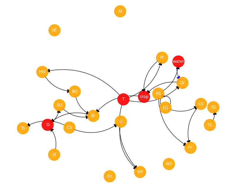
Interacting processes with memory effects are addressed in Section 2.3. These include environment-driven dependencies (such as interactions involving crop and grievance G, while selected interactions involving T and water were already defined in Section 2.1) and damage-mediated cascading effects, where previous impacts modify subsequent system states (e.g., incremental power grid damage resulting in blackout BO).

2.2.2. Transition matrix encoding (event resolution)

IN CONSTRUCTION

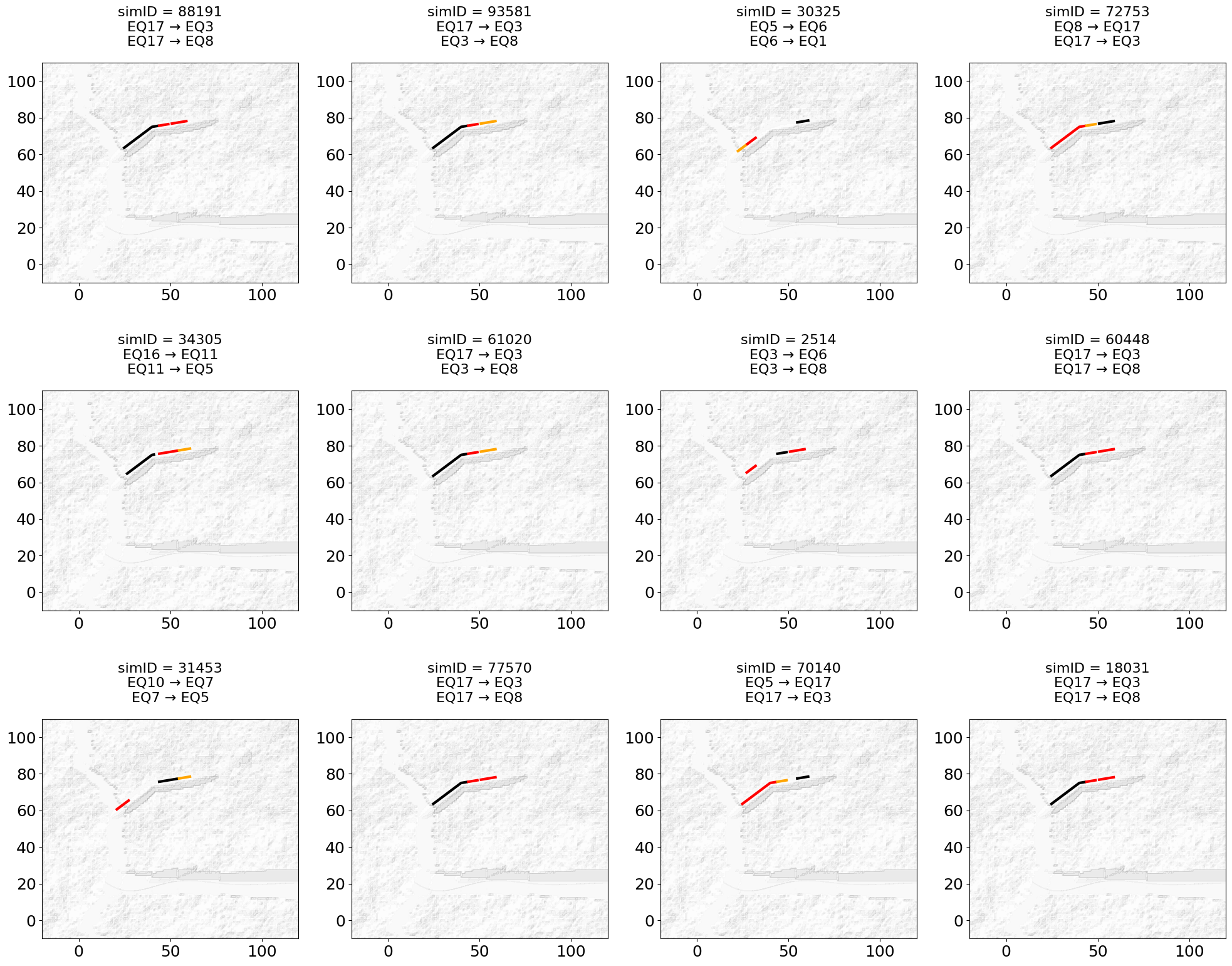
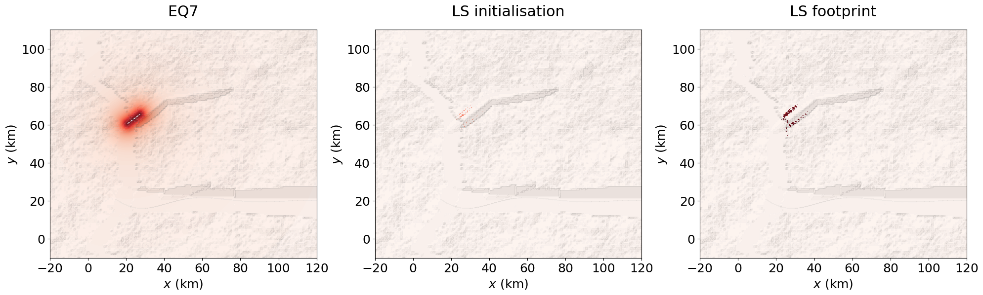
For v.1.2.1, only the earthquake EQ trigger case is considered to develop and demonstrate the computational framework. This case illustrates two types of one-to-one interactions: one governed by an analytically derived conditional probability, the other by a deterministic physical trigger.

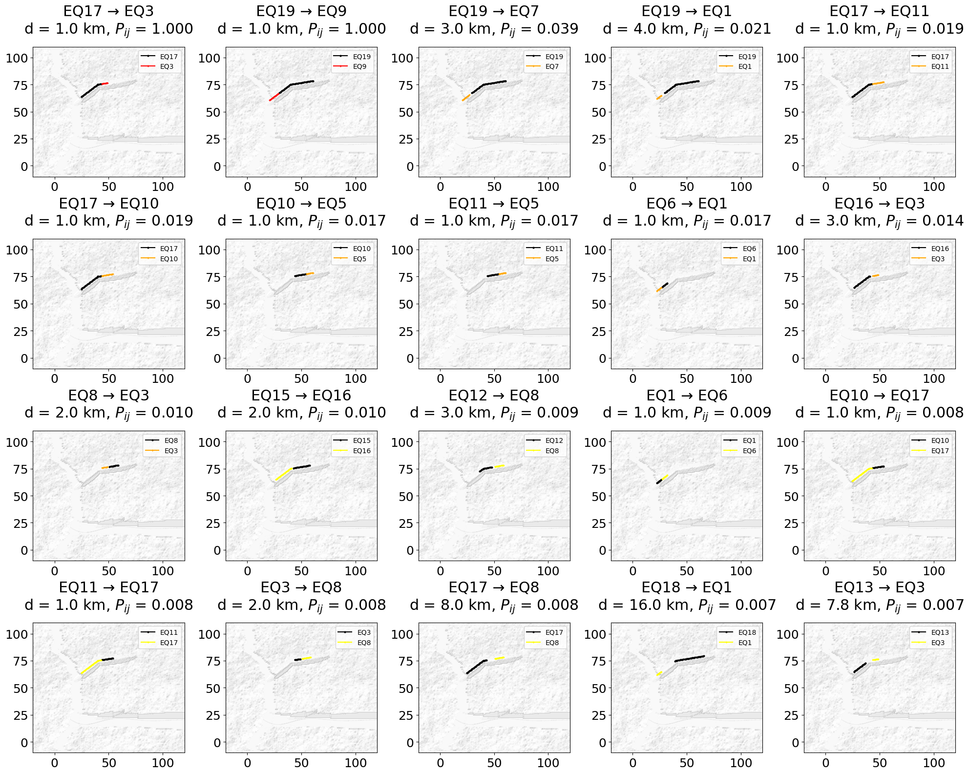
• EQ → EQ: Physical modelling of earthquake clustering is beyond the scope of the present project, as it would require dedicated Coulomb stress-transfer modelling tools. Instead, given the simplified geometry and the common reverse-faulting mechanism adopted in the model (see Tutorial 1 fault configuration), earthquake clusters are represented by allowing successive events to occur on the same fault, provided that their rupture areas do not overlap. Conditional probabilities of occurrence are calculated according to an analytical approximation of Coulomb stress transfer (Dieterich, 1994; Mignan, 2018:eq.6 - see calc_EQ_Dsigma()).

• EQ → LS: Earthquake-induced landslide initiation is represented using a Newmark sliding-block approach (Newmark, 1965). For each EQ event, the PGA footprint is combined with the local slope stability conditions to calculate the critical acceleration and the resulting permanent displacement using the empirical formulation of Jibson (2007). A displacement threshold is then applied to define the deterministic EQ-triggered LS initiation footprint. The triggered cells are subsequently propagated using CellularAutomaton_LS().

##################
## EQ → EQ CASE ##
##################

EQdyn_par = {'Dsig0_MPa': 1.,         # constant EQ stress drop (> 0)
             'dtau_dt_MPa_yr': 5e-3   # long-term tectonic stressing rate - tunable parameter
            }


ELT_EQ = ELT[ELT['ID'] == 'EQ']
EQi = ELT_EQ['evID'].values
n_EQ = len(EQi)
EQfault = ELT_EQ.set_index('evID')['srcID']

EQcoord = evchar[GenMR_perils.get_peril_evID(evchar['evID']) == 'EQ'].reset_index(drop = True)

EQrup = {
    evID: df[['x', 'y']].to_numpy()
    for evID, df in EQcoord.groupby('evID')
}

EQcluster = GenMR_dyn.get_evPairs_EQ(EQrup, EQfault)
EQ_p_ij = GenMR_dyn.fill_transitionMatrix_EQ(EQi, EQcluster, ELT_EQ, EQdyn_par, verbose = False)

print(EQ_p_ij.stack().sort_values(ascending=False).head(20))

EQ17  EQ3     1.000000
EQ19  EQ9     1.000000
      EQ7     0.038996
      EQ1     0.020519
EQ17  EQ10    0.018864
      EQ11    0.018864
EQ10  EQ5     0.016902
EQ11  EQ5     0.016902
EQ6   EQ1     0.016566
EQ16  EQ3     0.013604
EQ8   EQ3     0.010227
EQ15  EQ16    0.009767
EQ12  EQ8     0.009286
EQ1   EQ6     0.008777
EQ11  EQ17    0.008388
EQ10  EQ17    0.008388
EQ3   EQ8     0.008001
EQ17  EQ8     0.007838
EQ18  EQ1     0.007460
EQ13  EQ3     0.007422
dtype: float64

## plot main EQ pairs ##
EQcluster_plot = EQcluster.copy()
EQcluster_plot['p_ij'] = EQcluster_plot.apply(lambda row: EQ_p_ij.loc[row['trigger'], row['target']], axis=1)
EQcluster_plot = EQcluster_plot.sort_values('p_ij', ascending = False).head(20).reset_index(drop=True)

plt.rcParams['font.size'] = '18'
fig, ax = plt.subplots(4, 5, figsize=(20, 16))
ax = ax.flatten()
for i, row in EQcluster_plot.iterrows():
    ev1 = row['trigger']
    ev2 = row['target']
    rup1 = EQcoord[EQcoord['evID'] == ev1]
    rup2 = EQcoord[EQcoord['evID'] == ev2]
    p_ij = row['p_ij']

    if p_ij >= .9:
        target_color = 'red'         # almost certain triggering
    elif p_ij >= .1:
        target_color = 'darkorange'  # likely triggering
    elif p_ij >= .01:
        target_color = 'orange'      # possible triggering
    else:
        target_color = 'yellow'      # much less likely triggering

    ax[i].contourf(grid.xx, grid.yy, GenMR_env.ls.hillshade(topoLayer.z, vert_exag=.1), cmap='gray', alpha=.1)
    ax[i].plot(rup1['x'], rup1['y'], color='black',linewidth=1.5,marker='o',markersize=2,label=ev1,zorder=1)
    ax[i].plot(rup2['x'], rup2['y'], color=target_color, linewidth=1.5, marker='+', markersize=3, label=ev2,
        zorder=2)
    ax[i].set_xlim(grid.xmin, grid.xmax)
    ax[i].set_ylim(grid.ymin, grid.ymax)
    ax[i].set_aspect('equal')
    ax[i].set_title(
        f"{ev1} → {ev2}\n"
        f"d = {row['distance']:.1f} km, "
        f"$P_{{ij}}$ = {p_ij:.3f}", pad = 20)

    ax[i].legend(fontsize=10)

plt.tight_layout()

## update YET ##
Nsim = int(1e5)            # number of year-simulations, user-defined

## 1. Standard Poisson sampling
YLT_poi_EQ = GenMR_dyn.gen_YLT(ELT_EQ, Nsim, {'EQ': 'Poisson'})
YLT_poi_EQ['t'] = 0. + np.random.uniform(0, 1, size = len(YLT_poi_EQ))
YET_poi_EQ = YLT_poi_EQ[['simID', 'evID', 't']]  # remove loss for now...
                                                 # sampling reservoir of initial events, only 1st event to be kept

YET_dyn_EQ = GenMR_dyn.gen_YET_dyn_EQ(YET_poi_EQ, EQcluster, EQ_p_ij)

cluster_size = YET_dyn_EQ .groupby("simID") .size() .sort_values(ascending=False)

nrow, ncol = 3, 4
fig, ax = plt.subplots(nrow, ncol, figsize=(20, 16))
ax = ax.flatten()

colors = {
    0: 'black',        # original event
    1: 'red',          # first generation
    2: 'orange',       # second generation
    3: 'yellow'        # later generations if present
}

topN_sim = cluster_size.head(nrow*ncol).index
for k, simID in enumerate(topN_sim):
    axi = ax[k]
    cluster = YET_dyn_EQ[YET_dyn_EQ['simID'] == simID].sort_values('child')

    axi.contourf(grid.xx, grid.yy, GenMR_env.ls.hillshade(topoLayer.z, vert_exag = .1), cmap = 'gray', alpha = .1)

    for _, event in cluster.iterrows():
        ev = event['evID']
        child = event['child']
        rup = EQcoord[EQcoord['evID'] == ev]
        axi.plot(rup['x'], rup['y'], color = colors.get(child,'grey'), linewidth=3, zorder=child + 1)

    axi.set_xlim(grid.xmin, grid.xmax)
    axi.set_ylim(grid.ymin, grid.ymax)
    axi.set_aspect("equal")
    
    lines = []
    for _, row in cluster.iterrows():
        if not pd.isna(row['parent']):
            lines.append(f"{row['parent']} → {row['evID']}")
    chain = "\n".join(lines)
    axi.set_title(f"simID = {simID}\n{chain}", pad = 20, fontsize = 16)
plt.tight_layout();

##################
## EQ → LS CASE ##
##################

# test with one earthquake only to illustrate EQ-LS cellular automaton (not shown in tutorial 2)
# in the YET, if EQi occurs, LSi occurs at t+eps

EQtrigger = 'EQ7'
EQtrigger_fp = catalog_fp_haz[EQtrigger]                     # PGA (m/s2)
EQtrigger_coord = EQcoord[EQcoord['evID'] == EQtrigger]


hw = 0.                                   # water column (m)
wetness = hw / soilLayer.h
wetness[wetness > 1] = 1                  # max possible saturation
wetness[soilLayer.h == 0] = 0             # no soil case

movie = {'create': True, 'xmin': 15, 'xmax': 90, 'ymin': 30, 'ymax': 90}

LS_CA = GenMR_perils.CellularAutomaton_LS(soilLayer, wetness, movie, kmax = 10, trigger = 'EQ', amax = EQtrigger_fp)
LS_CA.run()
LS_CA.write_gif()
LS_footprint_hmax = LS_CA.result() 


# plot
Imax = 6 
Itrigger_plt = np.copy(EQtrigger_fp)
Itrigger_plt[Itrigger_plt >= Imax] = Imax

plt.rcParams['font.size'] = '18'
fig, ax = plt.subplots(1, 3, figsize=(20, 7))

ax[0].contourf(grid.xx, grid.yy, Itrigger_plt, cmap = 'Reds', levels = np.linspace(0, Imax, 100), 
               vmin=0, vmax=Imax)
ax[0].contourf(grid.xx, grid.yy, GenMR_env.ls.hillshade(topoLayer.z, vert_exag=.1), cmap='gray', alpha = .1)
ax[0].plot(EQtrigger_coord['x'], EQtrigger_coord['y'], color = 'white', linewidth = 1, linestyle = 'dashed')
ax[0].set_xlim(grid.xmin, grid.xmax)
ax[0].set_ylim(grid.ymin, grid.ymax)
ax[0].set_xlabel('$x$ (km)')
ax[0].set_ylabel('$y$ (km)')
ax[0].set_title(EQtrigger, pad = 20)
ax[0].set_aspect(1)

LS_fp0 = np.zeros((grid.nx, grid.ny))
FS = GenMR_env.calc_FS(soilLayer.topo.slope, soilLayer.h, wetness, soilLayer.par)
slope = np.radians(soilLayer.topo.slope)
ac = np.maximum((FS - 1) * 9.81 * np.sin(slope), 0)
amax = EQtrigger_fp
Dn = GenMR_perils.CellularAutomaton_LS._calc_newmark_jibson2007(amax, ac)
LS_fp0[Dn > 5] = 1                    # 5 cm threshold - initiates LS where slope is unstable

ax[1].pcolormesh(grid.xx, grid.yy, LS_fp0, cmap = 'Reds', vmin=0, vmax=2)
ax[1].contourf(grid.xx, grid.yy, GenMR_env.ls.hillshade(topoLayer.z, vert_exag=.1), cmap='gray', alpha = .1)
ax[1].set_xlim(grid.xmin, grid.xmax)
ax[1].set_ylim(grid.ymin, grid.ymax)
ax[1].set_xlabel('$x$ (km)')
ax[1].set_ylabel('$y$ (km)')
ax[1].set_title('LS initialisation', pad = 20)
ax[1].set_aspect(1)

ax[2].pcolormesh(grid.xx, grid.yy, LS_footprint_hmax, cmap = 'Reds', vmin=0, vmax=2)
ax[2].contourf(grid.xx, grid.yy, GenMR_env.ls.hillshade(topoLayer.z, vert_exag=.1), cmap='gray', alpha = .1)
ax[2].set_xlim(grid.xmin, grid.xmax)
ax[2].set_ylim(grid.ymin, grid.ymax)
ax[2].set_xlabel('$x$ (km)')
ax[2].set_ylabel('$y$ (km)')
ax[2].set_title('LS footprint', pad = 20)
ax[2].set_aspect(1)

plt.tight_layout();

iteration 10 / 10

# COMING LATER (v.1.2.3): all possible peril-peril interactions to be defined here + combination in YLT_dyn

2.3. Event interaction modelling (Non-Markovian process integration)

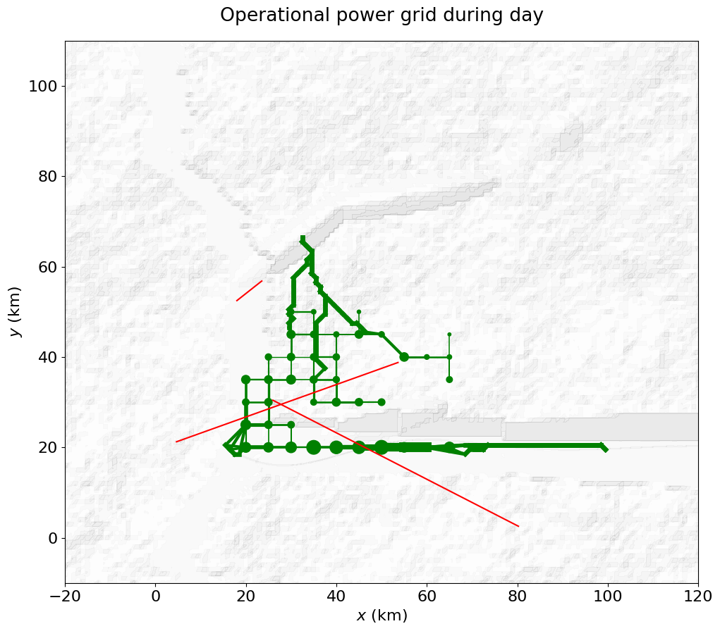
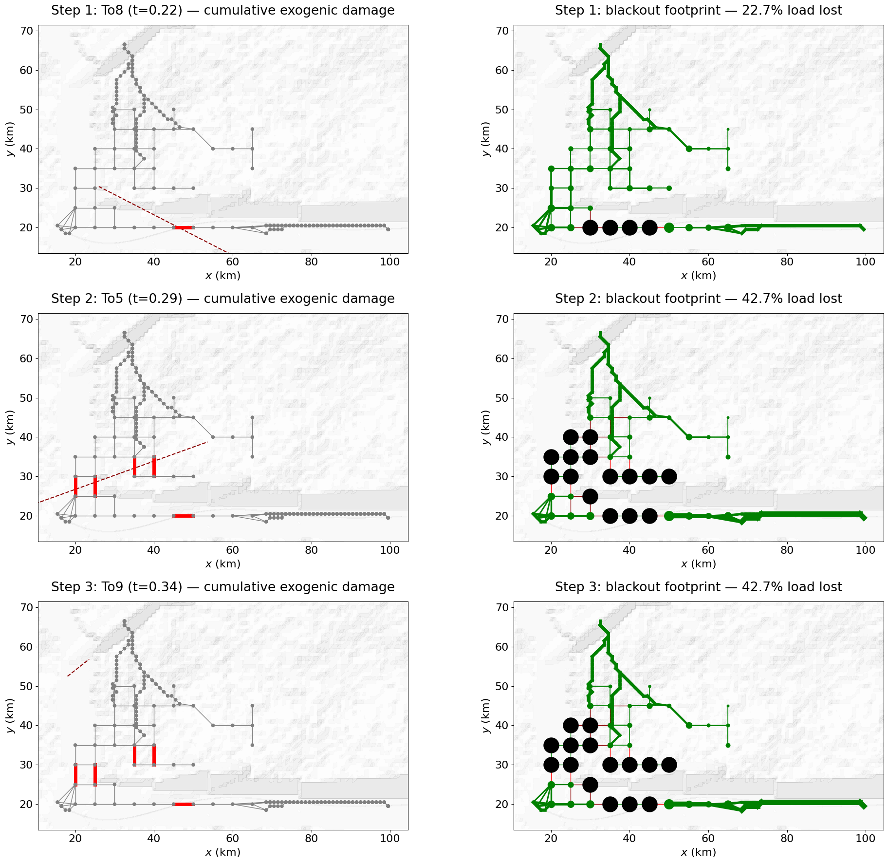
This section introduces memory into the dynamic YET, making the process explicitly non-Markovian. As a first worked example (v.1.2.1), we apply this to successive tornado To events cutting power grid transmission lines, with damage accumulating chronologically across the simulated year rather than resetting between events (i.e., no reparation). At each step, flow is recomputed on the currently damaged topology and cascading blackout BO is assessed. We expect early tornadoes to cause minor, localized loss of service, while later events striking an already-weakened grid trigger disproportionately larger blackouts, the signature of memory in the process.

##################
## To → BO CASE ##
##################

## Simulated tornados ##
ELT_To = ELT[ELT['ID'] == 'To']
Toi = ELT_To['evID'].values
n_To = len(Toi)

Tocoord = evchar[GenMR_perils.get_peril_evID(evchar['evID']) == 'To'].reset_index(drop = True)

# adhoc simulation year to test role of cumulative damage of tornados on power grid
n_trigger = 3
np.random.seed(9)   #3
YET_To = pd.DataFrame({'simID': np.ones(n_trigger), 
                       'evID': np.random.choice(Toi, size=n_trigger, replace=False)})

seasonal_par = {'To': {'peak_day': 130, 'kappa': 5}}   # early May, narrower season
YET_To['t'] = GenMR_dyn.sample_seasonal_t(seasonal_par['To']['peak_day'], seasonal_par['To']['kappa'], n_trigger)
YET_To = YET_To.sort_values('t').reset_index(drop=True)



## power grid ##
period = 'day'                       # 'day' or 'night'

powergrid_g, node_names, node_coords, node_supply = energyLayer.powergrid
node_names_list = [node_names[i] for i in range(len(node_names))]
indL = [i for i, name in node_names.items() if name.startswith('L')]
indS = [i for i, name in node_names.items() if name.startswith('S')]
indG = [i for i, name in node_names.items() if name.startswith('G')]
node_coords = np.array(node_coords)
L_coords = node_coords[indL]
S_coords = node_coords[indS]
G_coords = node_coords[indG]
edges = list(powergrid_g.edges())
slack_id = next(i for i, name in node_names.items() if name.startswith('Gdam'))

if period == 'day':
    node_served = energyLayer.node_served_day
    node_demand = energyLayer.node_demand_served_day
else:
    node_served = energyLayer.node_served_night
    node_demand = energyLayer.node_demand_served_night




## plot tornados vs power grid ##
plt.rcParams['font.size'] = 16
fig, ax = plt.subplots(1,1, figsize=(20, 10))

s_node, s_maxsupply, s_BO = 20, 200, 500
eps = 5
xmin_BO, xmax_BO = node_coords[:, 0].min() - eps, node_coords[:, 0].max() + eps
ymin_BO, ymax_BO = node_coords[:, 1].min() - eps, node_coords[:, 1].max() + eps


## Operational power grid ##
scale_factor = s_maxsupply / node_served[indL].max()
load_sizes = node_served[indL] * scale_factor

flows_op = energyLayer._compute_flows_dc(powergrid_g, node_supply, node_demand, slack_id = slack_id)[0]
edge_width_op = []
for i, j in edges:
    f = abs(flows_op.get((i,j), flows_op.get((j,i), 0.0)))
    # scale for plotting, max width = 10
    edge_width_op.append(1 + 9*f/np.max(list(flows_op.values())))

ax.contourf(grid.xx, grid.yy, GenMR_env.ls.hillshade(topoLayer.z, vert_exag=.1), cmap = 'gray', alpha = .1)
for (i,j), w in zip(edges, edge_width_op):
    ax.plot([node_coords[i,0], node_coords[j,0]],
                 [node_coords[i,1], node_coords[j,1]],
                 color='green', linewidth=w)
ax.scatter(L_coords[:,0], L_coords[:,1], color='green', s=load_sizes)
#for i, (x, y) in enumerate(node_coords):
#    ax.text(x + 1, y + 1, node_names[i], fontsize=8, zorder=3)
    
for evid in YET_To['evID'].unique():
    track = Tocoord[Tocoord['evID'] == evid].sort_values('x')
    ax.plot(track['x'], track['y'], color = 'red')

ax.set_xlabel('$x$ (km)')
ax.set_ylabel('$y$ (km)')
ax.set_title(f'Operational power grid during {period}', pad=20)
ax.set_aspect(1)
ax.set_xlim(grid.xmin, grid.xmax)
ax.set_ylim(grid.ymin, grid.ymax);

# demonstrate role of cumulative damage on BO emergence (assuming no reparation)

src.par['BO']['tolerance'] = 2       # high value to correct simplified topology (more redundancies in reality)
                                     # and lack of protection systems present in reality
                                     # value of 2 from trial and error, rare cascades when 1 element removed


        
from shapely.geometry import LineString, Point

def get_failed_edges(track_df, node_coords, node_names, edges):
    track_line = LineString(track_df[['x', 'y']].values)
    failed_lines = []
    for i, j in edges:
        edge_line = LineString([node_coords[i], node_coords[j]])
        if track_line.crosses(edge_line) or track_line.intersects(edge_line):
            failed_lines.append((node_names[i], node_names[j]))
    return failed_lines



n_nodes = len(node_names)
failed_lines_cum = set()
results = []

for step, row in YET_To_sorted.iterrows():
    evid, t = row['evID'], row['t']
    track = Tocoord[Tocoord['evID'] == evid]

    new_lines = get_failed_edges(track, node_coords, node_names, edges)

    failed_lines_cum.update(new_lines)
    failed_lines_step = list(failed_lines_cum)

    BO_loads, g_BO, g_dmg, g_intact, node_served_BO, node_supply_dmg = GenMR_perils.run_BO_flow(
        energyLayer, src.par['BO'], [], failed_lines_step,
        slack_id=slack_id, period=period, print_casc=False
    )

    frac_lost = 1 - node_served_BO[indL].sum() / node_served[indL].sum()

    print(f"[{step+1}/{len(YET_To_sorted)}] evID={evid}, t={t:.0f} | "
          f"new: {len(new_lines)} lines | "
          f"cum: {len(failed_lines_cum)} lines | "
          f"BO loads: {len(BO_loads)} | load lost: {frac_lost:.1%}")

    results.append(dict(
        step=step, evID=evid, t=t,
        failed_lines_cum=failed_lines_step.copy(),
        BO_loads=BO_loads, g_BO=g_BO, g_dmg=g_dmg, g_intact=g_intact,
        node_served_BO=node_served_BO, node_supply_dmg=node_supply_dmg,
        frac_lost=frac_lost
    ))

[1/3] evID=To8, t=0 | new: 1 lines | cum: 1 lines | BO loads: 4 | load lost: 22.7%
[2/3] evID=To5, t=0 | new: 4 lines | cum: 5 lines | BO loads: 15 | load lost: 42.7%
[3/3] evID=To9, t=0 | new: 0 lines | cum: 5 lines | BO loads: 15 | load lost: 42.7%

fraction_acceptable = .1   # if loss greater than 10%, shown in orange = brownout / partial supply


n_steps = len(results)
fig, axes = plt.subplots(n_steps, 2, figsize=(20, 6*n_steps))
if n_steps == 1:
    axes = axes.reshape(1, 2)   # keep 2D indexing consistent for a single row

for step, res in enumerate(results):
    ax_dmg = axes[step, 0]
    ax_bo  = axes[step, 1]

    failed_nodes = []
    failed_lines = res['failed_lines_cum']
    g_dmg = res['g_dmg']
    g_BO  = res['g_BO']
    node_served_BO = res['node_served_BO']
    node_supply_dmg = res['node_supply_dmg']
    BO_loads = res['BO_loads']

    A_dmg = GenMR_utils.graph_to_full_adjacency(g_dmg, n_nodes)

    ## exogenic (cumulative) damage ##
    edge_col_dmg = np.array(['grey' if A_dmg[i,j]==1 else 'red' for i,j in edges])
    edge_lw_dmg  = np.array([1 if A_dmg[i,j]==1 else 5 for i,j in edges])
    node_col_dmg = np.array(['red' if node_names[i] in failed_nodes else 'grey' for i in range(n_nodes)])
    node_s_dmg   = np.array([10*s_node if node_names[i] in failed_nodes else s_node for i in range(n_nodes)])

    ax_dmg.contourf(grid.xx, grid.yy, GenMR_env.ls.hillshade(topoLayer.z, vert_exag=.1),
                     cmap='gray', alpha=0.1)
    for (i,j), color, lw in zip(edges, edge_col_dmg, edge_lw_dmg):
        ax_dmg.plot([node_coords[i,0], node_coords[j,0]],
                    [node_coords[i,1], node_coords[j,1]], color=color, linewidth=lw)
    ax_dmg.scatter(node_coords[:,0], node_coords[:,1], color=node_col_dmg, s=node_s_dmg, zorder=2)

    track = Tocoord[Tocoord['evID'] == res['evID']]
    ax_dmg.plot(track['x'], track['y'], color='darkred', linewidth=1.5, linestyle='--', zorder=1)

    ax_dmg.set_xlabel('$x$ (km)')
    ax_dmg.set_ylabel('$y$ (km)')
    ax_dmg.set_title(f"Step {step+1}: {res['evID']} (t={res['t']:.2f}) — cumulative exogenic damage", pad=15)
    ax_dmg.set_aspect(1)
    ax_dmg.set_xlim(xmin_BO, xmax_BO)
    ax_dmg.set_ylim(ymin_BO, ymax_BO)

    ## Blackout footprint ##
    fraction_served = (node_served_BO[indL] - node_demand[indL]) / node_demand[indL]
    load_nodes = [node_names[i] for i in indL]
    load_col_BO = np.array([
        'black' if name in BO_loads else
        'darkorange' if fraction_served[i] < -fraction_acceptable else
        'green'
        for i, name in enumerate(load_nodes)
    ])
    load_s_BO = scale_factor * node_served_BO[indL]
    load_s_BO = np.array([s_BO if name in BO_loads else load_s_BO[i] for i, name in enumerate(load_nodes)])

    edge_col_BO = []
    for i, j in edges:
        in_BO  = (i, j) in g_BO.edges()  or (j, i) in g_BO.edges()
        in_dmg = (i, j) in g_dmg.edges() or (j, i) in g_dmg.edges()
        if not in_dmg:
            edge_col_BO.append('red')
        elif not in_BO:
            edge_col_BO.append('darkred')
        else:
            edge_col_BO.append('green')

    flows_BO = energyLayer._compute_flows_dc(g_BO, node_supply_dmg, node_demand, slack_id=slack_id)[0]
    edge_width_BO = []
    for i, j in edges:
        f = abs(flows_BO.get((i,j), flows_BO.get((j,i), 0.0)))
        edge_width_BO.append(1 + 9*f/np.max(list(flows_op.values())))

    ax_bo.contourf(grid.xx, grid.yy, GenMR_env.ls.hillshade(topoLayer.z, vert_exag=.1),
                   cmap='gray', alpha=0.1)
    for (i,j), color, w in zip(edges, edge_col_BO, edge_width_BO):
        ax_bo.plot([node_coords[i,0], node_coords[j,0]],
                   [node_coords[i,1], node_coords[j,1]], color=color, linewidth=w)
    for i, c, s in zip(indL, load_col_BO, load_s_BO):
        ax_bo.scatter(node_coords[i,0], node_coords[i,1], color=c, s=s, zorder=2)

    ax_bo.set_xlabel('$x$ (km)')
    ax_bo.set_ylabel('$y$ (km)')
    ax_bo.set_title(f"Step {step+1}: blackout footprint — {res['frac_lost']:.1%} load lost", pad=15)
    ax_bo.set_aspect(1)
    ax_bo.set_xlim(xmin_BO, xmax_BO)
    ax_bo.set_ylim(ymin_BO, ymax_BO)

plt.tight_layout();

3. Long-term drivers (coming later)

The framework introduced above is unchanged when extended to long-term drivers: the same Yearly Event Table (YET), or Yearly Loss Table (YLT) once loss modelling is included, is generated by simulating Nsim independent years. What changes is not the computational structure but the reference point in time: peril and/or vulnerability parameters are no longer evaluated under present-day conditions, but are instead conditioned on a specified target year in the far future (e.g. yr = 2075), so that the same generator can be reused for long-term change scenarios without modification to its stochastic engine.

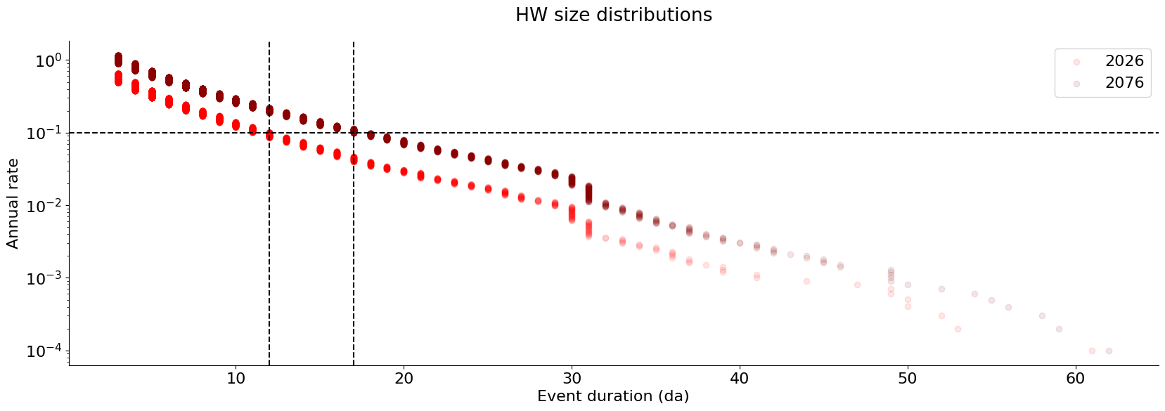
For v.1.2.1, this is demonstrated for global warming only, applying a simple linear trend to the present-day temperature T baseline.

COMING LATER (v.1.2.3): will include global warming, structure ageing…

# run sec. 2.1.1 first

yr_now = 2026
n_yr = 50
yr_future = yr_now + n_yr

globalwarming_rate = .025  #°C/year
T_rise = globalwarming_rate * n_yr
T0_future = T0 + T_rise
T_future = T + T_rise
print(f'Temperature increase of {T_rise}°C from {yr_now} to {yr_future}')

YET_HW_globalwarming, _, _ = GenMR_dyn.gen_YET_HW(T0_future, T_future, src.par['HW'], DT_peryr, DT_adv_daily, Nsim)


## event size distributions ##
S_HW, Sdistr_HW = GenMR_utils.calc_Sdistr_empirical(YET_HW, 'S')
S_HW_globalwarming, Sdistr_HW_globalwarming = GenMR_utils.calc_Sdistr_empirical(YET_HW_globalwarming, 'S')

RP = 10.   # yr
Srp_HW = np.interp(RP, 1 / Sdistr_HW, S_HW)
Srp_HW_globalwarming = np.interp(RP, 1 / Sdistr_HW_globalwarming, S_HW_globalwarming)

print(f"The {RP}-yr return period moves from a {Srp_HW:.0f}-day heatwave "
      f"to a {Srp_HW_globalwarming:.0f}-day heatwave under global warming.")

fig, ax = plt.subplots(1,1, figsize=(20, 6))
ax.scatter(S_HW, Sdistr_HW, color = 'red', alpha = .1, label = str(yr_now))
ax.scatter(S_HW_globalwarming, Sdistr_HW_globalwarming, color = 'darkred', alpha = .1, label = str(yr_future))
ax.axhline(1/RP, color = 'black', linestyle = 'dashed')
ax.axvline(Srp_HW, color = 'black', linestyle = 'dashed')
ax.axvline(Srp_HW_globalwarming, color = 'black', linestyle = 'dashed')
ax.set_yscale('log')
ax.set_xlabel('Event duration (da)')
ax.set_ylabel('Annual rate')
ax.set_title('HW size distributions', pad = 20)
ax.spines['right'].set_visible(False)
ax.spines['top'].set_visible(False)
ax.legend();

Temperature increase of 1.25°C from 2026 to 2076
The 10.0-yr return period moves from a 12-day heatwave to a 17-day heatwave under global warming.

References

• Dieterich, J.H. (1994). A constitutive law for rate of earthquake production and its application to earthquake clustering. Journal of Geophysical Research, 99(B2), 2601-2618.

• Jibson, R.W. (2007). Regression models for estimating coseismic landslide displacement. Engineering Geology, 91(2–4), 209–218.

• Mignan, A. (2018). Utsu aftershock productivity law explained from geometric operations on the permanent static stress field of mainshocks. Nonlinear Processes in Geophysics, 25, 241-250.

• Newmark, N.M. (1965). Effects of Earthquakes on Dams and Embankments. Géotechnique, 15(2), 139–160.