Tutorial 2: Implementing perils in the GenMR digital template
Author: Arnaud Mignan, Mignan Risk Analytics GmbH
Version: 1.2.1
Last Updated: 2026-07-07
License: AGPL-3
Once a virtual environment has been generated (see previous tutorial), stochastic events are modelled to populate it. Table 1 lists the perils included in version 1.1.2.
ID |
Peril |
Peril type† |
Source class |
Event size |
Intensity class |
Intensity measure |
Status‡ |
|---|---|---|---|---|---|---|---|
NATURAL |
|||||||
|
Asteroid impact |
Primary |
Point |
Kinetic energy (kt) |
Analytical |
Overpressure (kPa) |
✓ |
|
Convertive storm |
Primary (invisible\(^*\)) |
Area |
Cloud top height (km) |
Uniform |
Cloud top height (km) |
✓ |
|
Drought |
Primary (invisible\(^*\)) |
Area |
Duration (mon) |
Threshold |
Yes/no |
✓ |
|
Earthquake |
Primary |
Line |
Magnitude |
Analytical |
Peak ground acceleration (m/s\(^2\)) |
✓ |
|
Fluvial flood |
Secondary (to |
Point |
Peak flow |
Cellular automaton |
Inundation depth (m) |
✓ |
|
Heatwave |
Primary (invisible\(^*\)) |
Area |
Duration (da) |
Threshold |
Inside/outside |
✓ |
|
Lightning |
Secondary (to |
Point |
- |
- |
Yes/no |
✓ |
|
Landslide |
Secondary (to |
Diffuse |
Area (km\(^2\)) |
Cellular automaton |
Thickness (m) |
✓ |
|
Pest infestation |
Primary (invisible\(^*\)) |
Area |
Mean norm. population size |
Analytical |
Normalised population size |
✓ |
|
Rainstorm |
Primary (invisible\(^*\)) |
Area |
Rain intensity (mm/hr) |
Uniform |
Rain intensity (mm/hr) |
✓ |
|
Storm surge |
Secondary (to |
Line |
Coastal surge height (m) |
Threshold |
Inundation depth (m) |
✓ |
|
Tropical cyclone |
Primary |
Track |
Max. wind speed (m/s) |
Analytical |
Max. wind speed (m/s) |
✓ |
|
Tornado |
Primary |
Line |
Enhanced Fujita (EF) scale |
Analytical |
Max. wind speed (m/s) |
✓ |
|
Volcanic eruption |
Primary |
Point |
Volume erupted (km\(^3\)) |
Analytical |
Ash load (kPa) |
✓ |
|
Wildfire |
Primary |
Diffuse |
Burnt area |
Cellular automaton |
Burnt/not burnt |
✓ |
|
Windstorm |
Primary |
Area |
Max. wind speed (m/s) |
Uniform |
Max. wind speed (m/s) |
✓ |
TECHNOLOGICAL |
|||||||
|
Blackout |
Secondary (to |
Diffuse (network) |
Power loss (MW) |
Threshold |
Power loss (MW) |
✓ |
|
Explosion (industrial) |
Secondary (to |
Point |
TNT mass (kt) |
Analytical |
Overpressure \(P\) (kPa) |
✓ |
SOCIO-ECONOMIC |
|||||||
|
Business interruption |
Secondary (to |
Point |
- |
Threshold |
BI loss |
✓ |
|
Public safety service failure |
Secondary (to |
Point |
- |
Threshold |
Service loss |
✓ |
|
Social unrest |
Secondary (to |
Diffuse |
High grievance area |
Hybrid cellular automaton |
Burnt/not burnt |
✓ |
\(^*\) An event that does not cause any direct damage to buildings, at least in the present framework (following Mignan et al., 2014). Still implemented as triggering mechanism.
† Most perils are considered primary perils in this tutorial for sake of simplicity. Several will be considered secondary perils in Tutorial 3.
‡ Included in current version (✓), planned for v.1.1.2 (✗).
This tutorial is divided into two main sections. The first introduces the definition of peril sources, an event table (containing each event’s identifier and annual rate), and a corresponding catalogue of hazard-intensity footprints. The second section covers probabilistic risk assessment, in which damage and loss footprints are generated for each event identifier (Fig. 1) and risk metrics are calculated. Before beginning these sections, the digital-template environment created in the previous tutorial is loaded.
WARNING: This tutorial is intended solely to demonstrate how events and their footprints are generated. As such, only a very limited number of event sizes are considered for each peril as part of a model validation exercise. This is not sufficient for a robust risk assessment. For comprehensive risk analyses based on simulations spanning thousands to millions of years, see Tutorial 3 (currently under development).
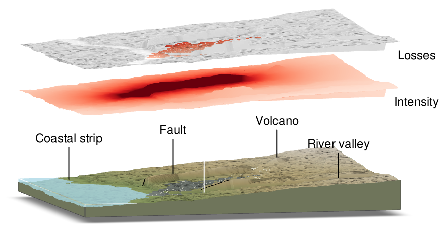
Fig. 1. One instance of the GenMR digital template (default parameterisation) with an example of event hazard intensity footprint and loss footprint (here for a large earthquake). Simulation rendered using Rayshader (Morgan-Wall, 2022).
import numpy as np
import pandas as pd
import copy
import matplotlib.pyplot as plt

import warnings
warnings.filterwarnings('ignore')   # commented, try to remove all warnings

from GenMR import perils as GenMR_perils
from GenMR import environment as GenMR_env
from GenMR import utils as GenMR_utils


# load inputs (i.e., outputs from Tutorial 1)
file_src = 'src.pkl'
file_topoLayer = 'envLayer_topo.pkl'
file_atmoLayer = 'envLayer_atmo.pkl'
file_soilLayer = 'envLayer_soil.pkl'
file_urbLandLayer = 'envLayer_urbLand.pkl'
file_energyLayer = 'envLayer_energy.pkl'
file_socioecoLayer = 'envLayer_socioeco.pkl'
src = GenMR_utils.load_pickle2class('/io/' + file_src)
grid = copy.copy(src.grid)
topoLayer = GenMR_utils.load_pickle2class('/io/' + file_topoLayer)
atmoLayer = GenMR_utils.load_pickle2class('/io/' + file_atmoLayer)
soilLayer = GenMR_utils.load_pickle2class('/io/' + file_soilLayer)
urbLandLayer = GenMR_utils.load_pickle2class('/io/' + file_urbLandLayer)
energyLayer = GenMR_utils.load_pickle2class('/io/' + file_energyLayer)
socioecoLayer = GenMR_utils.load_pickle2class('/io/' + file_socioecoLayer)

GenMR_env.plot_EnvLayers([topoLayer, atmoLayer, soilLayer, urbLandLayer, energyLayer,
                          socioecoLayer], file_ext = 'jpg', topo_bool = True)
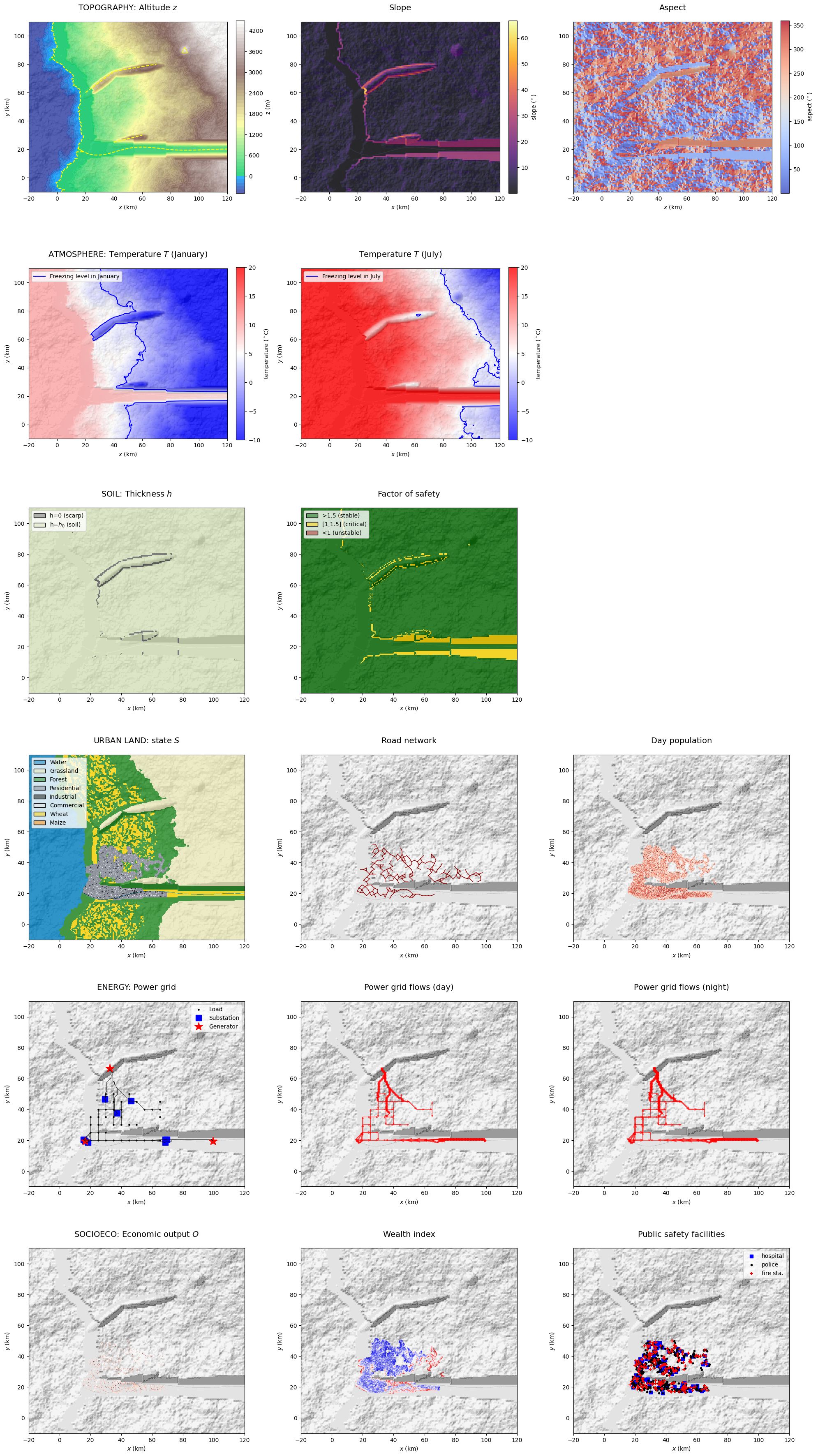
Note that the configuration of the digital template environment may be changed through Tutorial 1.
1. Stochastic event set
A list of stochastic events is defined, consisting of both primary and secondary events. Because event interactions will be addressed in the next tutorial, only simple ad-hoc one-to-one interactions are introduced here to illustrate how secondary event footprints can be generated (e.g., a storm surge from a tropical cyclone or a landslide triggered by a rainstorm). Conditional probabilities of occurrence will be examined in Tutorial 3. In this tutorial, only primary events have assigned annual rates.
1.1. Peril source definition
Source characteristics for earthquakes, volcanic eruptions, and fluvial floods were defined in Tutorial 1, as some environmental layers depend directly on these perils. Additional peril sources are now introduced.
WARNING: Only perils listed in src.par['perils'] will be modelled. The following perils require long computation times (minutes to tens of minutes on the first run; subsequent runs load from cache): Ex, FF, HW, LS, WF.
src.par['perils'] = ['AI','Dr','EQ','HW','PI','RS','TC','To','VE','WF','WS',        # primary
                     'CS',                                                          # special
                     'BI','BO','Ex','FF','Li','LS','Sf','SS','SU']                  # secondary
                    # IMPORTANT: primary perils come first in src.par['perils']
                    # NB: since 'CS' depends of 'To', must be listed after 'To' (i.e., CS=special peril)


src.par['rdm_seed'] = 42                          # None or integer (for stochastic sources: AI, TC)
if 'To' not in src.par['perils'] and 'CS' in src.par['perils']:
    # convective storm char. depend on tornado char.
    src.par['perils'].remove('CS')

# define new perils ('EQ', 'FF', 'VE' already initiated in Tutorial 1)
## NATURAL ##
src.par['AI'] = {'object': 'impact', 'N': 10}     # random uniform asteroid impacts (point sources)
src.par['CS'] = {'object': 'supercell',           # as trigger of lightnings and tornadoes
                 'R_km': 10.,                     # path conditioned on tornado path (better constrained)
                 'dH_CS2tropopause_km': 1.,       # distance between cloud top and tropopause (km)
                 'lat_deg': grid.par['lat_deg'],
                 'vforward_m/s': 20.              # forward storm speed (m/s)
                }
src.par['CS']['S'] = atmoLayer.z_tropopause - src.par['CS']['dH_CS2tropopause_km'] # size as cloud top height (km)
src.par['Dr'] = {'object': 'soil',
                 'hw_th': .1,                     # 10% of normal soil water content hw_fc_m
                 'Si_mo': [3, 6, 9],              # Fixed event sizes (months) - for sake of illustration
                 'sigmaT_yearly': .55,            # Temp. std. dev. - value from Olonscheck et al. (2021)
                 'lat_deg': grid.par['lat_deg']}
src.par['HW'] = {'object': 'atmosphere',
                 'T_th': 35.,                     # Minimum temperature threshold (°C)
                 'Dt_da': 3,                      # Minimum duration (days)
                 'Si_da': [7, 14],                # Fixed event sizes (days) - for sake of illustration
                 'sigmaT_yearly': .55,            # Temp. std. dev. - value from Olonscheck et al. (2021)
                 'T_AR1': [.9, 1.2],              # AR(1) process 0: corr. phi, 1: std dev (fitted west EU...)
                 'Dt_max_da': 30,                 # for Tutorial 2: HW defined over a month max
                 'month': 7,                      # Calendar month (July = 7) when heatwave occurrence explored
                 'lat_deg': grid.par['lat_deg']}
src.par['Li'] = {'object': 'supercell'}
src.par['LS'] = {'object': 'terrain'}
src.par['PI'] = {'object': 'crops',
                 'Si_yieldloss': [50,65],         # event size def. as mean crop loss %tage in entire region
                 'sigmaT_yearly': .55,            # Temp. std. dev. - value from Olonscheck et al. (2021)
                 'month': 7,                      # Calendar month (July = 7) when pest occurrence explored
                 'Tmin_compute': 30.,             # Minimum temperature (°C) to compute PI emergence
                 'lat_deg': grid.par['lat_deg'],
                 'landuse': urbLandLayer.S.copy()}
src.par['RS'] = {'object': 'atmosphere',          # as trigger of landslides
                 'duration': 24}                  # (hr) to calc. soil wetness that triggers LS & FF discharge
                                                  # somewhat ad-hoc, see Tutorial 3 for heavy rain (HR) model

src.par['SS'] = {'object': 'coastline'}
SS_src_xi, SS_src_yi = topoLayer.coastline_coord
src.SS_char = {'x': SS_src_xi, 'y': SS_src_yi}

src.par['TC'] = {'object': 'stormtrack', 'N': 5,  # pseudo-random track sources moving from West to East
                 'npt': 10,      # number of points along track, which crosses the grid from West to East
                 'max_dev': 3,   # random uniform deviation along the y-axis at each track point
                 'bin_km': 1.}   # track spatial resolution

src.par['To'] = {'object': 'vortexline', 'N': 9,  # random uniform vortex-line initiation points
                 'seed_xmax': 30.,                # initiates within [xmin+xbuffer, seed_xmax], i.e. warmer area
                 'theta_var': 45.,                # maximum angle deviation (°) from West-East direction
                 # beta distributions for stoch. line lengths function of EF size (3 defined: EF-3, EF-4, EF-5)
                 'L_alpha_beta_Lmax_EF3': [.744, 2.87, 100.],
                 'L_alpha_beta_Lmax_EF4': [1.077, 2.36, 100.],
                 'L_alpha_beta_Lmax_EF5': [1.222, 1.767, 100.],
                 'bin_km': 1.}   # line spatial resolution

src.par['WF'] = {'object': 'forest'}
src.par['WS'] = {'object': 'atmosphere'}          # area source instead of track source due to lack of simple model
                                                  # constant vmax for all (x,y) reasonable because grid small

## TECHNOLOGICAL ##
src.par['BO'] = {'object': 'power grid',
                 'tolerance': 2,                  # tolerance to overload (≥ 0)
                 'min_capacity_MW': 1.}           # minimum powergrid branch capacity
CI_x, CI_y = energyLayer.CI_refinery.centroid
src.par['Ex'] = {'object': 'refinery', 'N': 1, 'x': CI_x, 'y': CI_y}  # harbor refinery as source of explosions


## SOCIO-ECONOMIC ##
src.par['BI'] = {'object': 'urban footprint',     # WARNING: business restriction not considered, just BI
                                                  #          and only direct BI (not Leontief I-O propagation)
                 # from COM/IND building damage
                 'MDR_th': [.2, .9],              # BI threshold (ON/OFF): On above min. value
                 'daysOFF_MDR': [7., 6*30],       # duration from min. val. for min MDR_th to max. for max MDR_th
                                                  # NB: above max MDR_th, building has to be rebuilt
                 # from blackout
                 'daysOFF_gridNode_dmg': 30,      # time to repair one damaged power grid node
                 'daysOFF_gridLine_dmg_perkm': 1, # time to repair one km of damaged power line
                 'daysOFF_gridLine_trip': 1/24    # time to reset one tripped power line
                }
src.par['BI']['daysOFF_gridLine_dmg'] = src.par['BI']['daysOFF_gridLine_dmg_perkm'] * \
                                        energyLayer.par['powergrid_load_spacing_km']
# NB for later: max 'days_OFF_MDRi' could be function of management quality level (longer if bad)

src.par['Sf'] = {'object': 'urban footprint',
                 'MDR_th': .6}                    # Sf when CIs (e.g., hospitals) when buildings heavily damaged
src.par['SU'] = {'object': 'population',
                 ## seed ##
                 'Maslow_w': [.2,.3,.5],          # weights for job loss, safety loss, food loss
                 'wealth_alpha': 5,               # ≥1 exponent for sensitivity factor (1-wealth_index)**alpha
                                                  #      higher = grievance more concentrated in poor areas
                 'G1_decay_km': 30.,              # spatial decay length (km) for job loss grievance
                                                  #      (commute distance, labour catchment area)
                 'G2_decay_km': 10.,              # spatial decay length (km) for service access grievance
                                                  #      (emergency service reach)
                 'BI2jobloss_mon_th': 3,          # min. BI duration (in months) after which loss of job occurs
                 ## event propagation ##
                 'G_th': .2,                      # minimum grievance to initiate SU
                 'R_reach_km': 3.,                # max distance (km) of social unrest reach from unrest area
                 'max_iter': 5,                   # after how many blocks destroyed, unrest stopped by police
                                                  # (if not faster by natural SU die-off)
                 'plot_steps': True
                }

GenMR_perils.plot_src(src, hillshading_z = topoLayer.z, file_ext = 'jpg')
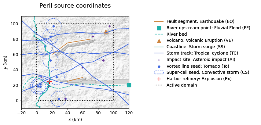
NOTE: Hazard intensity footprints are modeled based on the sources shown in the map above. For stochastic sources (AI, TC, To), rerunning the previous cell will produce different configurations unless rdm_seed is fixed. For To, the full stochastic source (line) can only be parameterised in EventSetGenerator() since its length depends on the event size distribution.
1.2. Event table generation
The stochastic event set (or event table) consists of a list of events per peril, with identifier evID, size S, and rate \(\lambda\) (lbd). Two types of perils are considered: primary perils for which the rate of occurrence must be assessed and secondary perils which will be assumed in this tutorial to occur in pair with their triggers (with rate NaN - for conditional probabilities, see the future Tutorial 3):
Primary perils:
AI,EQ,RS,TC,To,VE,WF,WS.Special perils:
CS(primary peril depending on characteristics ofTosecondary peril),Dr(rate calculated independently fromcalc_lbd_Dr()),HWandPI(rate derived from intensity footprint generation)Secondary perils:
Litriggered byCS,LSandFFtriggered byRS,SStriggered byTC,Extriggered by damage.
Event size distributions are parameterised in the dictionary sizeDistr with:
Event size incrementation according
Smin,SmaxandSbinwith binning inlinearorlogscale.Event size distribution modelled by one of 3 functions: power-law (
powerlaw, Mignan, 2024:eq. 2.38), exponential law (exponential, Mignan, 2024:eq. 2.39), or Generalised Pareto Distribution (GPD, Mignan, 2024:eq. 2.50).Rates of the digital template are for most perils simply calibrated by taking the ratio of the region area to the area used to obtain event productivity parameters in the Mignan (2024) textbook (e.g., global or continental United States, CONUS). This is a simplification assuming a homogeneous spatial distribution of events but is used as a straightforward way to define rates for the present virtual region. Contradictions may also arise, such as between tropical cyclones (TC) and windstorms (WS), which are not expected to occur within the same latitude range. However, the purpose of this tutorial is to define and illustrate all possible perils. The mutual exclusivity of TC and WS in the same region will be addressed in Tutorial 3. If you wish to avoid this issue in the current tutorial, simply remove either
TCorWSfromsizedistr['primary']- possible improvement: include latitude dependence of peril rate).
All calculations take place in the EventSetGenerator() class.
NOTE 1: The maximum possible event size, Smax, is defined by the user for all perils except earthquakes. For earthquakes, the maximum magnitude is constrained by the maximum fault length (src.EQ_char['srcMmax']) according to an empirical relationship (Mignan, 2024:fig. 2.6b).
NOTE 2: A floating rupture approach is used to generate earthquake ruptures on existing fault segments. See Appendix B to visualise the stochastic ruptures created by running the next cell, and refer to the Reference Manual for details on the method.
NOTE 3: The number of stochastic events is set equal to the number of sources when the sources themselves are stochastic (i.e., AI, TC). This number is kep very low for illustration purposes.
NOTE 4: The rate of heatwaves (HW) and of pest infestations (PI) is computed jointly with the generation of their intensity footprints, as their occurrence is governed by extremes in a stochastic spatiotemporal temperature field constrained by the atmospheric environmental layer.
NOTE 5: See Appendix C5 for the blackout (BO) case since it is a secondary invisible peril, which behaviour depends on the stochastic distribution of element failures. Idem for business interruption (BI), public safety service failure (Sf) and social unrest (SU) - see C.6-C.8.
EQ_Mmax = np.max(src.EQ_char['srcMmax'])

sizeDistr = {
    # WARNING: all src.par['perils'] modelled, do not remove perils below if listed in src.par['perils']
    'primary': ['AI','EQ','RS','TC','To','VE','WF','WS'],
    'special': ['CS','Dr','HW','PI'],
    'secondary': ['FF','Li','LS','SS', 'Ex'],
    # primary perils
    'AI':{
        'Nstoch': src.par['AI']['N'], 'Sunit': 'Bolide energy $E$ (kton)',
        'Smin': 10, 'Smax': 1e3, 'Sbin': 1, 'Sscale': 'log',
        'distr': 'powerlaw', 'region': 'global', 'a0': .5677, 'b': .9,      # see Mignan (2024:sect.2.3.1)
        'calibration_source': '',
        'reference': 'to_add'
    },
    'EQ':{
        'Nstoch': 20, 'Sunit': 'Magnitude',
        'Smin': 6, 'Smax': EQ_Mmax, 'Sbin': .1, 'Sscale': 'linear',
        'distr': 'exponential', 'a': 5, 'b': 1.,         # i.e., one M = a-value EQ per year (given b-value = 1)
        'calibration_source': 'user-defined',
        'reference': 'none'
    },
    'RS':{
        'Nstoch': 3, 'Sunit': 'Water column (mm/hr)',
        'Smin': 75, 'Smax': 125, 'Sbin': 25, 'Sscale': 'linear',
        'distr': 'GPD', 'region': 'CONUS', 'mu': 50., 'xi': -.051, 'sigma': 11.8, 'Lbdmin0': 522.,
            # see Mignan (2024:sect.2.3.2)
        'calibration_source': '',
        'reference': 'to_add'
    },
    'TC':{
        'Nstoch': src.par['TC']['N'], 'Sunit': 'Max. wind speed (m/s)',
        'Smin': 40, 'Smax': 65, 'Sbin': 10, 'Sscale': 'linear',
        'distr': 'GPD', 'region': 'global', 'mu': 33., 'xi': -.280, 'sigma': 17.8,'Lbdmin0': 43.9,
#        , 'Lbdmin': .1      # overwrites Lbdmin derived from Lbdmin0 to directly choose rate(>=Smin) = Lbdmin
        'calibration_source': 'IBTrACS',
        'reference': 'to_add'
    },
    'To':{
        'Nstoch': src.par['To']['N'], 'Sunit': 'Enhanced Fujita scale',
        'Smin': 3, 'Smax': 5, 'Sbin': 1, # WARNING: hardcoded, do not change, depends on 'L_alpha_beta_Lmax_EF*'
        'Sscale': 'linear',
        'distr': 'exponential', 'region': 'CONUS', 'a0': 3.6, 'b': .9,
        'calibration_source': 'NOAA 1950-2021 tornadoes (public)',
        'reference': 'to_add'
    },
    'VE':{
        'Nstoch': 3, 'Sunit': 'Ash volume (km$^3$)',
        'Smin': 1, 'Smax': 10, 'Sbin': .5, 'Sscale': 'log',
        'distr': 'powerlaw', 'region': 'global', 'a0': -1.155, 'b': .66,      # see Sect. 2.3.1
        'calibration_source': '',
        'reference': 'to_add'
    },
    'WF':{
        'Nstoch': 10, 'Sunit': 'Burnt area (ha)',
        'Smin': 1e4, 'Smax': 1e5, 'Sbin': .5, 'Sscale': 'log',
        'distr': 'powerlaw', 'region': 'global', 'a0': 8.553, 'b': 1.23,      # see Sect. 2.3.1
        'calibration_source': '',
        'reference': 'to_add'
    },
    'WS':{
        'Nstoch': 2, 'Sunit': 'Max. wind speed (m/s)',
        'Smin': 45, 'Smax': 50, 'Sbin': 5, 'Sscale': 'linear',
        'distr': 'GPD', 'region': 'local', 'mu': 17., 'xi': -.112, 'sigma': 4.43, 'Lbdmin': 163.25,
        # GPD params. for Brest (France) location for illustration purposes (consider making it func. of lat.)
        'calibration_source': 'Copernicus 1986-2011 Synthetic windstorm events for Europe',
        'reference': '10.24381/cds.ce973f02'
    },
    # special perils
    'CS':{                # CS triggers To but To param better constrained, backpropagating to CS
        'Nstoch': src.par['To']['N']
    },
    'Dr':{                # Dr event rates to be calculated in calc_lbd_Dr() - see next code cell
        'Nstoch': len(src.par['Dr']['Si_mo'])
    },
    'HW':{                # HW event rates to be calculated alongside footprint generation
        'Nstoch': len(src.par['HW']['Si_da'])
    },
    'PI':{                # PI event rates to be calculated alongside footprint generation
        'Nstoch': len(src.par['PI']['Si_yieldloss'])
    },
    # secondary perils - here ad-hoc Pr(peril|trigger) = 1, see tutorial 3 for probabilistic case
    'FF':{'trigger': 'RS'},
    'Li':{'trigger': 'CS'},
    'LS':{'trigger': 'RS'},
    'SS':{'trigger': 'TC'},
    'Ex':{'trigger': 'dg',     # 'dg' label indicates event triggered by damage caused by any peril (tutorial 3)
          'S': 1., 'Sunit': 'Explosive yield (kton)'
    }
}

eventSet = GenMR_perils.EventSetGenerator(src, sizeDistr, GenMR_utils)
evtable, evchar = eventSet.generate()

evchar.to_csv('io/evchar.csv', index = False)
#evtable
with pd.option_context('display.max_rows', None,
                       'display.max_columns', None):
    display(evtable)
| ID | srcID | evID | S | lbd | |
|---|---|---|---|---|---|
| 0 | AI | impact1 | AI1 | 10.000000 | 2.657777e-06 |
| 1 | AI | impact2 | AI2 | 10.000000 | 2.657777e-06 |
| 2 | AI | impact3 | AI3 | 10.000000 | 2.657777e-06 |
| 3 | AI | impact4 | AI4 | 100.000000 | 2.509457e-07 |
| 4 | AI | impact5 | AI5 | 100.000000 | 2.509457e-07 |
| 5 | AI | impact6 | AI6 | 100.000000 | 2.509457e-07 |
| 6 | AI | impact7 | AI7 | 100.000000 | 2.509457e-07 |
| 7 | AI | impact8 | AI8 | 1000.000000 | 4.212292e-08 |
| 8 | AI | impact9 | AI9 | 1000.000000 | 4.212292e-08 |
| 9 | AI | impact10 | AI10 | 1000.000000 | 4.212292e-08 |
| 10 | Dr | soil | Dr1 | 3.000000 | NaN |
| 11 | Dr | soil | Dr2 | 6.000000 | NaN |
| 12 | Dr | soil | Dr3 | 9.000000 | NaN |
| 13 | EQ | fault1 | EQ1 | 6.000000 | 6.855726e-03 |
| 14 | EQ | fault2 | EQ2 | 6.000000 | 6.855726e-03 |
| 15 | EQ | fault1 | EQ3 | 6.000000 | 6.855726e-03 |
| 16 | EQ | fault1 | EQ4 | 6.100000 | 5.445696e-03 |
| 17 | EQ | fault1 | EQ5 | 6.100000 | 5.445696e-03 |
| 18 | EQ | fault1 | EQ6 | 6.100000 | 5.445696e-03 |
| 19 | EQ | fault1 | EQ7 | 6.200000 | 6.488506e-03 |
| 20 | EQ | fault1 | EQ8 | 6.200000 | 6.488506e-03 |
| 21 | EQ | fault1 | EQ9 | 6.300000 | 3.436002e-03 |
| 22 | EQ | fault1 | EQ10 | 6.300000 | 3.436002e-03 |
| 23 | EQ | fault1 | EQ11 | 6.300000 | 3.436002e-03 |
| 24 | EQ | fault1 | EQ12 | 6.400000 | 4.093970e-03 |
| 25 | EQ | fault1 | EQ13 | 6.400000 | 4.093970e-03 |
| 26 | EQ | fault2 | EQ14 | 6.500000 | 3.251956e-03 |
| 27 | EQ | fault1 | EQ15 | 6.500000 | 3.251956e-03 |
| 28 | EQ | fault1 | EQ16 | 6.600000 | 5.166241e-03 |
| 29 | EQ | fault1 | EQ17 | 6.700000 | 4.103691e-03 |
| 30 | EQ | fault1 | EQ18 | 6.800000 | 3.259678e-03 |
| 31 | EQ | fault1 | EQ19 | 6.900000 | 2.589254e-03 |
| 32 | EQ | fault1 | EQ20 | 7.000000 | 2.056718e-03 |
| 33 | HW | atmosphere | HW1 | 7.000000 | NaN |
| 34 | HW | atmosphere | HW2 | 14.000000 | NaN |
| 35 | PI | crops | PI1 | 50.000000 | NaN |
| 36 | PI | crops | PI2 | 65.000000 | NaN |
| 37 | RS | atmosphere | RS1 | 75.000000 | 1.000793e-03 |
| 38 | RS | atmosphere | RS2 | 100.000000 | 8.172054e-05 |
| 39 | RS | atmosphere | RS3 | 125.000000 | 4.562873e-06 |
| 40 | TC | stormtrack1 | TC1 | 40.000000 | 2.841439e-04 |
| 41 | TC | stormtrack2 | TC2 | 50.000000 | 1.637893e-04 |
| 42 | TC | stormtrack3 | TC3 | 60.000000 | 4.064719e-05 |
| 43 | TC | stormtrack4 | TC4 | 60.000000 | 4.064719e-05 |
| 44 | TC | stormtrack5 | TC5 | 70.000000 | 3.110718e-05 |
| 45 | To | vortexline1 | To1 | 3.000000 | 4.537519e-05 |
| 46 | To | vortexline2 | To2 | 3.000000 | 4.537519e-05 |
| 47 | To | vortexline3 | To3 | 3.000000 | 4.537519e-05 |
| 48 | To | vortexline4 | To4 | 4.000000 | 5.712399e-06 |
| 49 | To | vortexline5 | To5 | 4.000000 | 5.712399e-06 |
| 50 | To | vortexline6 | To6 | 4.000000 | 5.712399e-06 |
| 51 | To | vortexline7 | To7 | 5.000000 | 7.191484e-07 |
| 52 | To | vortexline8 | To8 | 5.000000 | 7.191484e-07 |
| 53 | To | vortexline9 | To9 | 5.000000 | 7.191484e-07 |
| 54 | VE | volcano1 | VE1 | 1.000000 | 7.303024e-07 |
| 55 | VE | volcano1 | VE2 | 3.162278 | 3.415881e-07 |
| 56 | VE | volcano1 | VE3 | 10.000000 | 1.597728e-07 |
| 57 | WF | forest | WF1 | 10000.000000 | 1.062953e-02 |
| 58 | WF | forest | WF2 | 10000.000000 | 1.062953e-02 |
| 59 | WF | forest | WF3 | 10000.000000 | 1.062953e-02 |
| 60 | WF | forest | WF4 | 10000.000000 | 1.062953e-02 |
| 61 | WF | forest | WF5 | 10000.000000 | 1.062953e-02 |
| 62 | WF | forest | WF6 | 10000.000000 | 1.062953e-02 |
| 63 | WF | forest | WF7 | 31622.776602 | 5.158744e-03 |
| 64 | WF | forest | WF8 | 31622.776602 | 5.158744e-03 |
| 65 | WF | forest | WF9 | 31622.776602 | 5.158744e-03 |
| 66 | WF | forest | WF10 | 100000.000000 | 3.755478e-03 |
| 67 | WS | atmosphere | WS1 | 45.000000 | 2.741867e-03 |
| 68 | WS | atmosphere | WS2 | 50.000000 | 1.746819e-05 |
| 69 | CS | supercell | CS_toTo1 | 13.811900 | NaN |
| 70 | CS | supercell | CS_toTo2 | 13.811900 | NaN |
| 71 | CS | supercell | CS_toTo3 | 13.811900 | NaN |
| 72 | CS | supercell | CS_toTo4 | 13.811900 | NaN |
| 73 | CS | supercell | CS_toTo5 | 13.811900 | NaN |
| 74 | CS | supercell | CS_toTo6 | 13.811900 | NaN |
| 75 | CS | supercell | CS_toTo7 | 13.811900 | NaN |
| 76 | CS | supercell | CS_toTo8 | 13.811900 | NaN |
| 77 | CS | supercell | CS_toTo9 | 13.811900 | NaN |
| 78 | Ex | refinery | Ex_fromCIf | 1.000000 | NaN |
| 79 | FF | river1 | FF_fromRS1 | NaN | NaN |
| 80 | FF | river1 | FF_fromRS2 | NaN | NaN |
| 81 | FF | river1 | FF_fromRS3 | NaN | NaN |
| 82 | Li | supercell | Li_fromCS1 | NaN | NaN |
| 83 | Li | supercell | Li_fromCS2 | NaN | NaN |
| 84 | Li | supercell | Li_fromCS3 | NaN | NaN |
| 85 | Li | supercell | Li_fromCS4 | NaN | NaN |
| 86 | Li | supercell | Li_fromCS5 | NaN | NaN |
| 87 | Li | supercell | Li_fromCS6 | NaN | NaN |
| 88 | Li | supercell | Li_fromCS7 | NaN | NaN |
| 89 | Li | supercell | Li_fromCS8 | NaN | NaN |
| 90 | Li | supercell | Li_fromCS9 | NaN | NaN |
| 91 | LS | terrain | LS_fromRS1 | NaN | NaN |
| 92 | LS | terrain | LS_fromRS2 | NaN | NaN |
| 93 | LS | terrain | LS_fromRS3 | NaN | NaN |
| 94 | SS | coastline | SS_fromTC1 | NaN | NaN |
| 95 | SS | coastline | SS_fromTC2 | NaN | NaN |
| 96 | SS | coastline | SS_fromTC3 | NaN | NaN |
| 97 | SS | coastline | SS_fromTC4 | NaN | NaN |
| 98 | SS | coastline | SS_fromTC5 | NaN | NaN |
Running the EventSetGenerator is effectively instantaneous. In contrast, computing drought (Dr) rates requires several minutes and is therefore executed as a separate step (see below). The calculation is based on a water-balance model in which soil water content evolves from an initial state (defined by the soil layer’s 'moisture_regime') and is subsequently modulated by evapotranspiration (see calc_PET()) and precipitation (see gen_precipitation()) over the twelve months of a calendar year. Conditions conducive to drought development arise during anticyclonic years, when accompanied by anomalously high summer temperatures.
Note: The correlation between Dr, HW, PI, and the anticorrelation with RS, will be examined in Tutorial 3.
## optional cell / better constrained in Tutorial 3 ##

rates_Dr = GenMR_perils.calc_lbd_Dr(src.par['Dr'], atmoLayer.par, soilLayer.par)
evtable.loc[evtable['evID'].str[:2] == 'Dr', 'lbd'] = rates_Dr
Simulating droughts: 100%|██████████| 1000000/1000000 [05:52<00:00, 2835.94it/s]
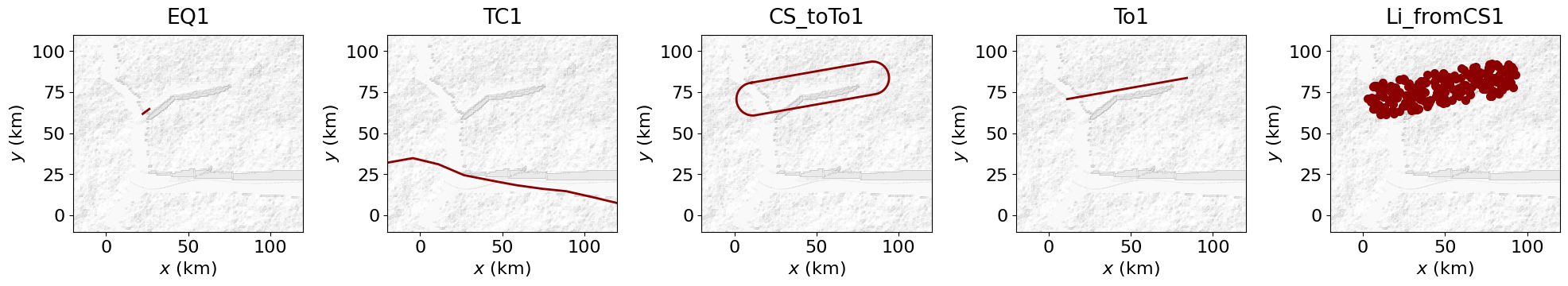
The evchar dataframe contains the coordinates of the events defined in evtable. The following code cell allows the user to plot stochastic events via their evID:
#print('total list of modelled events, by evID:', evtable['evID'].unique())

## SELECT EVENTS ##
evID_list = ['EQ1','TC1','CS_toTo1', 'To1','Li_fromCS1']
#evID_list = evtable['evID'].values
###################

n_evID = len(evID_list)

max_cols = 5
ncols = min(n_evID, max_cols)
nrows = int(np.ceil(n_evID / ncols))

evID_coords = evchar[evchar['evID'].isin(evID_list)].reset_index(drop = True)

plt.rcParams['font.size'] = '16'
fig, ax = plt.subplots(nrows, ncols, figsize=(4 * ncols, 4 * nrows), squeeze=False)
ax = ax.flatten()
for i in range(n_evID):
    peril_evID = evID_list[i][:2]
    if peril_evID in ['AI', 'VE', 'Li']:
        plot_type = 'scatter'
    elif  peril_evID in ['EQ', 'TC', 'To', 'CS', 'SS']:
        plot_type = 'plot'
    coords2plt = evID_coords[evID_coords['evID'] == evID_list[i]]
    ax[i].contourf(grid.xx, grid.yy, GenMR_env.ls.hillshade(topoLayer.z, vert_exag=.1), cmap='gray', alpha = .1)
    if plot_type == 'plot':
        ax[i].plot(coords2plt['x'], coords2plt['y'], color = 'darkred', linewidth = 2)
    elif plot_type == 'scatter':
        ax[i].scatter(coords2plt['x'], coords2plt['y'], color = 'darkred', linewidth = 2)
    ax[i].set_xlim(grid.xmin, grid.xmax)
    ax[i].set_ylim(grid.ymin, grid.ymax)
    ax[i].set_xlabel('$x$ (km)')
    ax[i].set_ylabel('$y$ (km)')
    ax[i].set_title(evID_list[i], pad = 10)
    ax[i].set_aspect(1)

for j in range(n_evID, len(ax)):
    ax[j].axis('off')

plt.tight_layout();
1.3. Intensity footprint catalogue generation
Once the event table has been generated, the next step is to produce one mean hazard-intensity footprint per event. Aleatory uncertainty is not implemented for simplicity, and because it does not affect the objectives of this project, namely, modelling compound events in a virtual environment (see the third and final tutorial).
NOTE: See Appendixes C.5-C.8 for the footprint modelling of blackouts (BO), business interruption (BI), public safety service failure (Sf) and social unrest (SU). Since they depend on too many potential initial conditions, illustrative scenarios are presented in the Appendix.
1.3.1. From analytical expressions & threshold models
1.3.1.1. Analytical expressions
Analytical expressions are available to calculate intensity \(I(x,y) = f_I(S,r)\) for the AI/Ex, EQ, VE and TC perils (Mignan, 2024:sec. 2.4.1). The size \(S\) is provided in evtable, while the distance-to-source \(r\) is obtained by matching each event to its corresponding source coordinates via evchar. Because generating TC footprints requires a multi-step procedure, additional details are provided in Appendix C.
The models are implemented as calc_I_*(S,r) functions in the Python file, using the equations from Mignan (2024:sec. 2.4.1):
ID |
Event size \(S\) |
Intensity \(I\) |
Equation |
|---|---|---|---|
|
Explosive mass \(m_{TNT}\) (kt) |
Blast overpressure \(P\) (kPa) |
Eq. 2.56 |
|
Magnitude \(M\) |
Peak ground acceleration PGA (m/s\(^2\)) |
Eq. 2.54 |
|
- |
Lightning strike count (/convective storm) |
to add |
|
Maximum wind speed \(v_{max}\) (m/s) |
Wind speed \(v\) (m/s) |
Eq. 2.24 |
|
Enhanced Fujita (EF) scale to max. wind speed (m/s) |
Max. wind speed \(v_{max}\) (m/s) |
Eq. 2.59 |
|
Erupted volume \(V\) (km\(^3\)) |
Ash load \(P\) (kPa), converted from thickness (m) |
Eq. 2.61 |
Note that the analytical expression of pest infestation (PI) intensity is of the form \(I(x,y) = f_I(T(x,y))\) with \(T(x,y)\) the near-surface air temperature in the digital template (eq. to add). The footprint is only defined for the land-use state \(S\) = 5 or 6 (crops: wheat or maize - see the model_PI_analytical() function).
1.3.1.2. Threshold models
Heatwave (
HW): Based on an event being declared when the near-surface air temperature equals or exceedsT_thfor at leastDt_daconsecutive days. Temperature extremes in the digital template arise from the combination of large-scale advective temperature anomalies and temporally correlated daily temperature variability (see themodel_HW_threshold()function). It should be noted that, for a given event sizeS, the largest spatial footprint (i.e., the most extreme realization) is selected from a larger stochastic event set (see all candidate footprints infigs/HW_stochset_tmp/).Storm surge (
SS): Based on the Bathtub model (Mignan, 2024:sec. 2.4.2). The algorithm is intentionally simple and tailored to the virtual environment used here, where the background topography exhibits a predominantly west-east gradient (see themodel_SS_Bathtub()function). As a secondary peril triggered byTCevents, theSSsize along the coastline is derived from a relationship of the form \(h_{max} \propto v_{max}^2\) (Mignan, 2024:fig. 2.7), where \(v_{max}\) is the wind speed along the coastline obtained from theTCfootprint.
Note that rainstorm (RS) and windstorm (WS) footprints are considered spatially homogeneous (prior to the application of any site-specific conditions, which will be addressed subsequently) due to the relatively small size of the active domain of the digital template. Accordingly, their source classes are defined as area sources, and their intensity classes are defined using thresholds, with the threshold value corresponding to the event size S by construction.
The catalogue of hazard footprints is generated via the HazardFootprintGenerator(() class and is visualised with plot_hazFootprints().
src.par['TC']['vforward_m/s'] = 10.         # forward storm speed (m/s)
src.par['TC']['pn_mbar'] = 1005.            # ambient pressure (mbar) - NB: consider using atm. layer p0
src.par['TC']['B_Holland'] = 2              # Holland's parameter (see Fig. 2.10 of textbook)
src.par['TC']['lat_deg'] = grid.lat_deg     # average latitude of digital template (see Tutorial 1)

src.par['To']['Rmax_m'] = 300.              # user-defined, independent of EF scale since no model available
                                            # high value used for illustration

# virtual region bathymetry characteristics for SS height given storm wind speed
src.par['SS']['bathy'] = 'New York harbor'  # 'generic' (Saffir-Simpson, Mignan, 2024:eq. 2.16)
                                            # 'New York harbor' (eq. in Mignan, 2024:fig. 2.7)

## TO ADD: site-specific conditions ##
# surface friction -> reduce windspeed (TC, WS)
# soil amplification -> increase ground shaking (EQ)
# urban heat island -> increase temperature (HW)
# other?

hazFootprints = GenMR_perils.HazardFootprintGenerator(evtable, evchar, src, topoLayer.z, atmoLayer)
catalog_hazFootprints = hazFootprints.generate()
generating footprints for: AI... Dr... EQ... HW... (loading from cache)
PI... (loading from cache)
RS... TC... To... VE... WF... WS... CS... BI... BO... Ex... FF... Li... LS... Sf... SS... SU... catalogue completed
# max intensity Imax in color range (see units in previous table)
# to compare similar levels of expected damage, choose a value per peril for a constant MDR in the vulnerability
# curves (see curves generated by plot_vulnFunctions())
Imax_Ex_totaldestruction = 4 * 6.89476  # kPa (here 4 psi as threshold of total destruction)

plot_Imax = {'AI': Imax_Ex_totaldestruction, 'EQ': 6, 'Ex': Imax_Ex_totaldestruction, \
             'HW': src.par['HW']['T_th'] + 5, 'LS': 2., 'PI': 1,\
             'SS': 2., 'TC': 70., 'To': 70., 'VE': .5, 'WS': 70.}
f = .1
plot_Imin = {'AI': f*plot_Imax['AI'], 'EQ': f*plot_Imax['EQ'], 'Ex': f*plot_Imax['Ex'], \
             'HW': src.par['HW']['T_th'], 'LS': f*plot_Imax['LS'], 'PI': 0, 'SS': f*plot_Imax['SS'], \
             'TC': 30., 'To': 30., 'VE': f*plot_Imax['VE'], 'WS': 30.}

# nstoch (default = 5) defines the number of events per peril to be displayed by row
# if the number of events > nstoch, footprints are randomly sampled from all possibilities
GenMR_perils.plot_hazFootprints(catalog_hazFootprints, grid, topoLayer.z, plot_Imin, plot_Imax)  #, nstoch = 5)
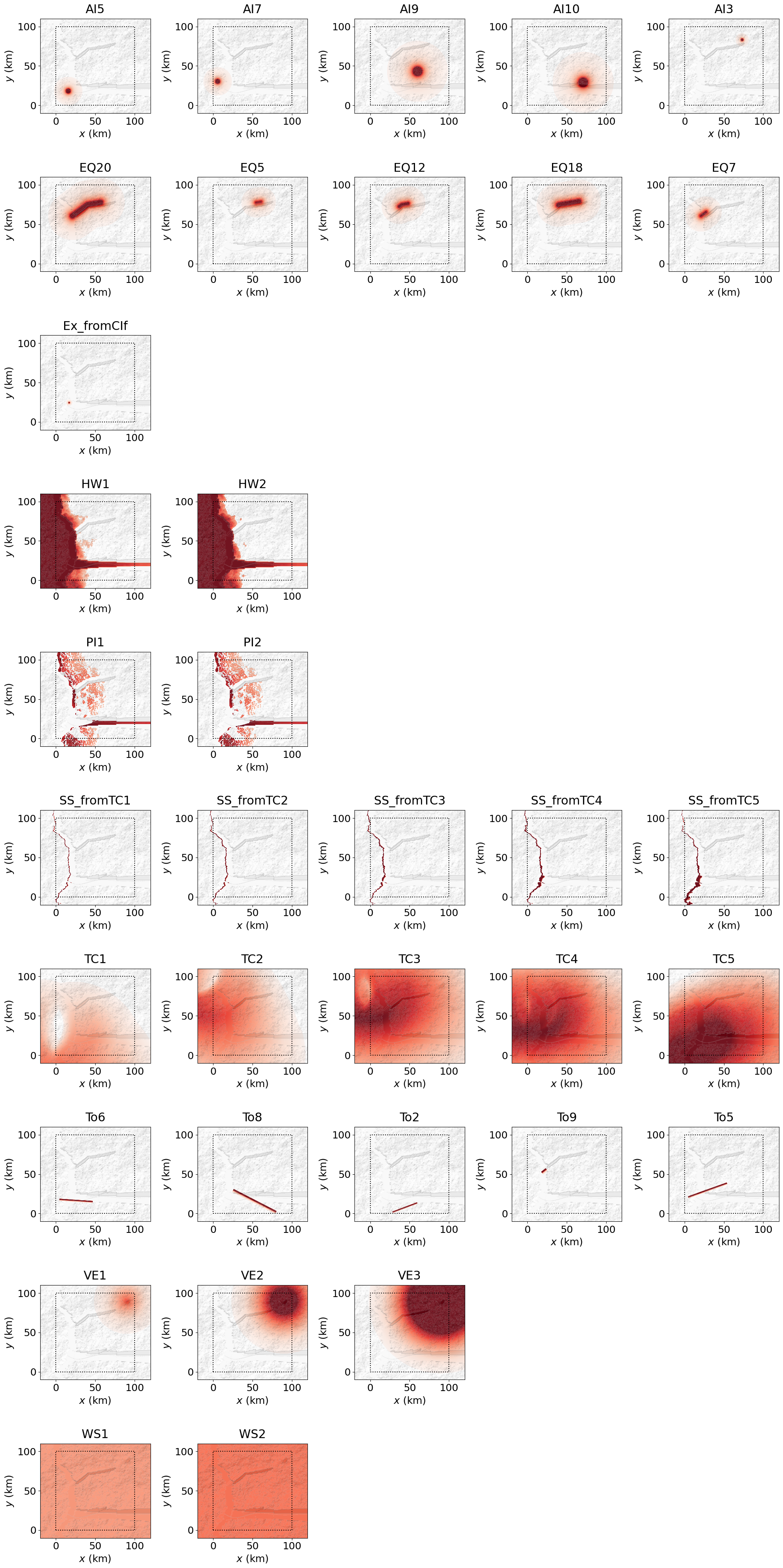
Note: Observe the TC footprint boundary effect (cyclonic eye), which is due to the track artificially starting at grid.xmin.
It was previously indicated that the HW and PI event rates are computed jointly with the generation of their intensity footprints. It is possible to retrieve these rates from:
rates_HW = hazFootprints.rate_HW
rates_PI = hazFootprints.rate_PI

# update event table
evtable.loc[evtable['evID'].str[:2] == 'HW', 'lbd'] = rates_HW
evtable.loc[evtable['evID'].str[:2] == 'PI', 'lbd'] = rates_PI

with pd.option_context('display.max_rows', None):
    display(evtable)
| ID | srcID | evID | S | lbd | |
|---|---|---|---|---|---|
| 0 | AI | impact1 | AI1 | 10.000000 | 2.657777e-06 |
| 1 | AI | impact2 | AI2 | 10.000000 | 2.657777e-06 |
| 2 | AI | impact3 | AI3 | 10.000000 | 2.657777e-06 |
| 3 | AI | impact4 | AI4 | 100.000000 | 2.509457e-07 |
| 4 | AI | impact5 | AI5 | 100.000000 | 2.509457e-07 |
| 5 | AI | impact6 | AI6 | 100.000000 | 2.509457e-07 |
| 6 | AI | impact7 | AI7 | 100.000000 | 2.509457e-07 |
| 7 | AI | impact8 | AI8 | 1000.000000 | 4.212292e-08 |
| 8 | AI | impact9 | AI9 | 1000.000000 | 4.212292e-08 |
| 9 | AI | impact10 | AI10 | 1000.000000 | 4.212292e-08 |
| 10 | Dr | soil | Dr1 | 3.000000 | NaN |
| 11 | Dr | soil | Dr2 | 6.000000 | NaN |
| 12 | Dr | soil | Dr3 | 9.000000 | NaN |
| 13 | EQ | fault1 | EQ1 | 6.000000 | 6.855726e-03 |
| 14 | EQ | fault2 | EQ2 | 6.000000 | 6.855726e-03 |
| 15 | EQ | fault1 | EQ3 | 6.000000 | 6.855726e-03 |
| 16 | EQ | fault1 | EQ4 | 6.100000 | 5.445696e-03 |
| 17 | EQ | fault1 | EQ5 | 6.100000 | 5.445696e-03 |
| 18 | EQ | fault1 | EQ6 | 6.100000 | 5.445696e-03 |
| 19 | EQ | fault1 | EQ7 | 6.200000 | 6.488506e-03 |
| 20 | EQ | fault1 | EQ8 | 6.200000 | 6.488506e-03 |
| 21 | EQ | fault1 | EQ9 | 6.300000 | 3.436002e-03 |
| 22 | EQ | fault1 | EQ10 | 6.300000 | 3.436002e-03 |
| 23 | EQ | fault1 | EQ11 | 6.300000 | 3.436002e-03 |
| 24 | EQ | fault1 | EQ12 | 6.400000 | 4.093970e-03 |
| 25 | EQ | fault1 | EQ13 | 6.400000 | 4.093970e-03 |
| 26 | EQ | fault2 | EQ14 | 6.500000 | 3.251956e-03 |
| 27 | EQ | fault1 | EQ15 | 6.500000 | 3.251956e-03 |
| 28 | EQ | fault1 | EQ16 | 6.600000 | 5.166241e-03 |
| 29 | EQ | fault1 | EQ17 | 6.700000 | 4.103691e-03 |
| 30 | EQ | fault1 | EQ18 | 6.800000 | 3.259678e-03 |
| 31 | EQ | fault1 | EQ19 | 6.900000 | 2.589254e-03 |
| 32 | EQ | fault1 | EQ20 | 7.000000 | 2.056718e-03 |
| 33 | HW | atmosphere | HW1 | 7.000000 | 5.100000e-03 |
| 34 | HW | atmosphere | HW2 | 14.000000 | 1.700000e-03 |
| 35 | PI | crops | PI1 | 50.000000 | 3.950000e-03 |
| 36 | PI | crops | PI2 | 65.000000 | 0.000000e+00 |
| 37 | RS | atmosphere | RS1 | 75.000000 | 1.000793e-03 |
| 38 | RS | atmosphere | RS2 | 100.000000 | 8.172054e-05 |
| 39 | RS | atmosphere | RS3 | 125.000000 | 4.562873e-06 |
| 40 | TC | stormtrack1 | TC1 | 40.000000 | 2.841439e-04 |
| 41 | TC | stormtrack2 | TC2 | 50.000000 | 1.637893e-04 |
| 42 | TC | stormtrack3 | TC3 | 60.000000 | 4.064719e-05 |
| 43 | TC | stormtrack4 | TC4 | 60.000000 | 4.064719e-05 |
| 44 | TC | stormtrack5 | TC5 | 70.000000 | 3.110718e-05 |
| 45 | To | vortexline1 | To1 | 3.000000 | 4.537519e-05 |
| 46 | To | vortexline2 | To2 | 3.000000 | 4.537519e-05 |
| 47 | To | vortexline3 | To3 | 3.000000 | 4.537519e-05 |
| 48 | To | vortexline4 | To4 | 4.000000 | 5.712399e-06 |
| 49 | To | vortexline5 | To5 | 4.000000 | 5.712399e-06 |
| 50 | To | vortexline6 | To6 | 4.000000 | 5.712399e-06 |
| 51 | To | vortexline7 | To7 | 5.000000 | 7.191484e-07 |
| 52 | To | vortexline8 | To8 | 5.000000 | 7.191484e-07 |
| 53 | To | vortexline9 | To9 | 5.000000 | 7.191484e-07 |
| 54 | VE | volcano1 | VE1 | 1.000000 | 7.303024e-07 |
| 55 | VE | volcano1 | VE2 | 3.162278 | 3.415881e-07 |
| 56 | VE | volcano1 | VE3 | 10.000000 | 1.597728e-07 |
| 57 | WF | forest | WF1 | 10000.000000 | 1.062953e-02 |
| 58 | WF | forest | WF2 | 10000.000000 | 1.062953e-02 |
| 59 | WF | forest | WF3 | 10000.000000 | 1.062953e-02 |
| 60 | WF | forest | WF4 | 10000.000000 | 1.062953e-02 |
| 61 | WF | forest | WF5 | 10000.000000 | 1.062953e-02 |
| 62 | WF | forest | WF6 | 10000.000000 | 1.062953e-02 |
| 63 | WF | forest | WF7 | 31622.776602 | 5.158744e-03 |
| 64 | WF | forest | WF8 | 31622.776602 | 5.158744e-03 |
| 65 | WF | forest | WF9 | 31622.776602 | 5.158744e-03 |
| 66 | WF | forest | WF10 | 100000.000000 | 3.755478e-03 |
| 67 | WS | atmosphere | WS1 | 45.000000 | 2.741867e-03 |
| 68 | WS | atmosphere | WS2 | 50.000000 | 1.746819e-05 |
| 69 | CS | supercell | CS_toTo1 | 13.811900 | NaN |
| 70 | CS | supercell | CS_toTo2 | 13.811900 | NaN |
| 71 | CS | supercell | CS_toTo3 | 13.811900 | NaN |
| 72 | CS | supercell | CS_toTo4 | 13.811900 | NaN |
| 73 | CS | supercell | CS_toTo5 | 13.811900 | NaN |
| 74 | CS | supercell | CS_toTo6 | 13.811900 | NaN |
| 75 | CS | supercell | CS_toTo7 | 13.811900 | NaN |
| 76 | CS | supercell | CS_toTo8 | 13.811900 | NaN |
| 77 | CS | supercell | CS_toTo9 | 13.811900 | NaN |
| 78 | Ex | refinery | Ex_fromCIf | 1.000000 | NaN |
| 79 | FF | river1 | FF_fromRS1 | NaN | NaN |
| 80 | FF | river1 | FF_fromRS2 | NaN | NaN |
| 81 | FF | river1 | FF_fromRS3 | NaN | NaN |
| 82 | Li | supercell | Li_fromCS1 | NaN | NaN |
| 83 | Li | supercell | Li_fromCS2 | NaN | NaN |
| 84 | Li | supercell | Li_fromCS3 | NaN | NaN |
| 85 | Li | supercell | Li_fromCS4 | NaN | NaN |
| 86 | Li | supercell | Li_fromCS5 | NaN | NaN |
| 87 | Li | supercell | Li_fromCS6 | NaN | NaN |
| 88 | Li | supercell | Li_fromCS7 | NaN | NaN |
| 89 | Li | supercell | Li_fromCS8 | NaN | NaN |
| 90 | Li | supercell | Li_fromCS9 | NaN | NaN |
| 91 | LS | terrain | LS_fromRS1 | NaN | NaN |
| 92 | LS | terrain | LS_fromRS2 | NaN | NaN |
| 93 | LS | terrain | LS_fromRS3 | NaN | NaN |
| 94 | SS | coastline | SS_fromTC1 | NaN | NaN |
| 95 | SS | coastline | SS_fromTC2 | NaN | NaN |
| 96 | SS | coastline | SS_fromTC3 | NaN | NaN |
| 97 | SS | coastline | SS_fromTC4 | NaN | NaN |
| 98 | SS | coastline | SS_fromTC5 | NaN | NaN |
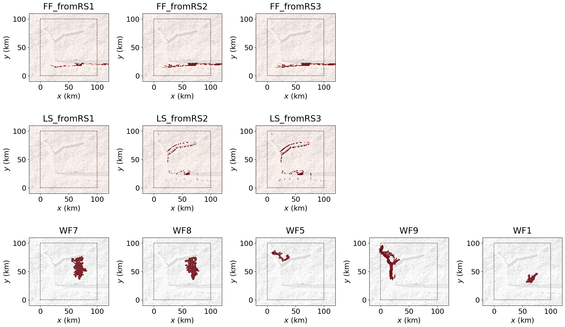
1.3.2. From numerical models (cellular automata)
Generation of hazard-intensity footprints via dynamical processes (here, cellular automata - CA) is handled separately because these computations are more expensive. This functionality is implemented in the DynamicHazardFootprintGenerator() class and applied to the LS, FF and WF perils. Details of the corresponding CA models can be found in the Python file within the CellularAutomaton_* classes, where * denotes the peril ID.
The following movie illustrates an example of dynamical process. It is produced by running LS_CA.write_gif() in the next cell and shows the time-evolving landslide propagation generated by the CA. The final hazard-intensity footprint included in the hazard-footprint catalogue is static and defined as \(\max_t I(x,y,t)\).
reproduce_LSmovie = False          # True to create 'movs/LS_CA_xrg38_68_yrg20_35.gif'
reproduce_FFmovie = False          # True to create 'movs/FF_CA_xrg0_100_yrg0_40.gif'

if reproduce_LSmovie:
    movie = {'create': True, 'xmin': 38, 'xmax': 68, 'ymin': 20, 'ymax': 35}   # zoom on specific hill

    evID_trigger = 'RS3'                                       # case considered for movie scenario
    S_trigger = evtable['S'][evtable['evID'] == evID_trigger].values
    S_trigger = 175 # TMP
    hw = S_trigger * 1e-3 * src.par['RS']['duration']          # water column (m)
    wetness = hw / soilLayer.h
    wetness[wetness > 1] = 1                                   # max possible saturation
    wetness[soilLayer.h == 0] = 0                              # no soil case

    LS_CA = GenMR_perils.CellularAutomaton_LS(soilLayer, wetness, movie)
    LS_CA.run()
    LS_CA.write_gif()
    print()
    print('LS movie created (go to mov/LS_CA_*).')
else:
    print('No LS movie created.')

if reproduce_FFmovie:
    I_RS = evtable[evtable['evID'] == 'RS3']['S'].values[0] * 1e-3 / 3600    # (mm/hr) to (m/s)
    movie = {'create': True, 'xmin': 0, 'xmax': 100, 'ymin': 0, 'ymax': 40, 'tmin': 40}

    FF_CA = GenMR_perils.CellularAutomaton_FF(I_RS, src, grid, topoLayer.z, movie)
    FF_CA.run()
    FF_CA.write_gif()
    print()
    print('FF movie created (go to mov/FF_CA_*).')
else:
    print('No FF movie created.')
No LS movie created.
No FF movie created.
Footprints are initialised in dynhazFootprints, an instance of the DynamicHazardFootprintGenerator() class. Running dynhazFootprints.generate() computes all dynamical intensity footprints at once. To generate only a specific subset of perils, one must use dynhazFootprints.generate(selected_perils = ['LS', 'FF', ...]). Note that if a peril has already been run, cached footprints will be loaded automatically. To force recomputation, one needs to include the option force_recompute = True in the class command (or delete the folder *_CA_frames).
# additional WF source/landuse parameters
src.par['WF'] = {'ratio_grass': .6,        # ratio of forest cells to turn to grass at initial state
             'p_lightning': .1,            # probability of lightning strike per iteration
             'rate_newtrees': 1000,        # number of new trees to add per iteration
             'nsim': 100000,               # number of iterations
             'Smin_plot': 1000,            # minimum WF footprint size to save in 'figs/WF_CA_frames'
            }

dynhazFootprints = GenMR_perils.DynamicHazardFootprintGenerator(evtable, src, soilLayer, urbLandLayer)
catalog_dynhazFootprints = dynhazFootprints.generate()
#_ = dynhazFootprints.generate(selected_perils = ['LS'], force_recompute = True)
#catalog_dynhazFootprints = dynhazFootprints.generate(selected_perils = ['FF'], force_recompute = True)
catalog_dynhazFootprints.keys()
generating footprints for:
Loading from cache potential footprints

Fetching footprints from potential footprints
Fetching WF footprints from cache: 100%|████████| 10/10 [00:00<00:00, 35.50it/s]
FF_fromRS1 (loaded from cache)
FF_fromRS2 (loaded from cache)
FF_fromRS3 (loaded from cache)
LS_fromRS1 (loaded from cache)
LS_fromRS2 (loaded from cache)
LS_fromRS3 (loaded from cache)
... catalogue completed
dict_keys(['WF1', 'WF2', 'WF3', 'WF4', 'WF5', 'WF6', 'WF7', 'WF8', 'WF9', 'WF10', 'FF_fromRS1', 'FF_fromRS2', 'FF_fromRS3', 'LS_fromRS1', 'LS_fromRS2', 'LS_fromRS3'])
try:
    plot_Imin.update({'LS': 0, 'FF': 0, 'WF': 0})
    plot_Imax.update({'LS': 2, 'FF': 1, 'WF': 1})
except NameError:
    plot_Imin = {'LS': 0, 'FF': 0, 'WF': 0}
    plot_Imax = {'LS': 2, 'FF': 1, 'WF': 1}

catalog_dynhazFootprints = dynhazFootprints.catalog_hazFootprints
GenMR_perils.plot_hazFootprints(catalog_dynhazFootprints, grid, topoLayer.z, plot_Imin, plot_Imax)
# merge the two catalogues
catalog_allhazFootprints = catalog_hazFootprints | catalog_dynhazFootprints

# update src class file for tutorial 3
GenMR_utils.save_class2pickle(src, filename = 'src')
# bypass dynamic footprints for rapid tests...
#catalog_allhazFootprints = catalog_hazFootprints
2. Probabilistic risk assessment
In this final section, loss footprints are modelled, and total losses per event are added as new column in the event table, creating an event loss table (ELT). Risk metrics are then calculated from the ELT (considering only primary events in this tutorial). Year loss tables will be addressed in the future Tutorial 3.
2.1. Vulnerability curve definition
Generic intensity-specific vulnerability functions, \(D = f_D(I)\), are implemented and apply to any building type for simplicity. The vulnerability functions (f_D()) are listed below and correspond to the equations described in Section 3.2.5 of Mignan (2024). Damage is expressed in terms of the mean damage ratio (MDR):
ID |
Intensity \(I\) |
Vulnerability function |
Parameters |
|---|---|---|---|
|
Blast overpressure \(P\) [kPa] |
Cum. lognormal distr. (Eq. 3.13) |
\(\mu\) = log(20), \(\sigma\) = 0.4 |
|
Peak ground acceleration PGA [m/s\(^2\)] |
Cum. lognormal distr. (Eq. 3.13) |
\(\mu\) = log(6), \(\sigma\) = 0.6 |
|
Inundation depth \(h\) [m] |
Square root (Eq. 3.10) |
\(c\) = 0.45 |
|
Landslide thickness \(h\) [m] |
Weibull distr. (Eq. 3.12) |
\(c_1\) = -1.671, \(c_2\) = 3.189, \(c_3\) = 1.746 |
|
Ash load \(P\) [kPa] (converted from thickness [m]) |
Cum. lognormal distr. (Eq. 3.13) |
\(\mu\) = 1.6, \(\sigma\) = 0.4 |
|
Maximum wind speed \(v_{max}\) [m/s] |
Power-law (Eq. 3.14) |
\(v_{thres}\) = 25.7, \(v_{half}\) = 74.7 |
|
Burnt yes/no |
Heaviside step function |
MDR = 1 if burnt, 0 otherwise |
GenMR_perils.plot_vulnFunctions()
2.2. Loss footprint catalogue generation
Damage footprints, \(D(x,y)\), are obtained by mapping hazard-intensity footprints, \(I(x,y)\), into mean damage ratio (MDR) values using the vulnerability functions defined earlier. Loss footprints, \(L(x,y)\), are calculated as the product of \(D(x,y)\) and the exposure footprint, \(\nu(x,y)\).
It should be noted that losses are computed for independent events occurring individually. For example, the total loss from a TC event could depend on losses caused by the associated SS event. Such interactions, whether at the exposure or damage level, will be addressed in Tutorial 3.
exposure_val = socioecoLayer.bldg_blockValue_modif   # corr. for wealth index (or urbLandLayer.bldg_BlockValue)
riskFootprints_all = GenMR_perils.RiskFootprintGenerator(catalog_allhazFootprints, exposure_val, evtable)
catalog_dmgFootprints = riskFootprints_all.catalog_dmgFootprints
catalog_lossFootprints = riskFootprints_all.catalog_lossFootprints

# ELT saved in folder 'io/' (an input of tutorial 3)
riskFootprints_all.ELT.to_parquet('io/ELT.parquet')

with pd.option_context('display.max_rows', None):
    display(riskFootprints_all.ELT)
Computing MDR & Loss: 100%|█████████████████████| 76/76 [00:01<00:00, 39.77it/s]
| ID | srcID | evID | S | lbd | loss | |
|---|---|---|---|---|---|---|
| 0 | AI | impact1 | AI1 | 10.000000 | 2.657777e-06 | 2.605143e+00 |
| 1 | AI | impact2 | AI2 | 10.000000 | 2.657777e-06 | 0.000000e+00 |
| 2 | AI | impact3 | AI3 | 10.000000 | 2.657777e-06 | 0.000000e+00 |
| 3 | AI | impact4 | AI4 | 100.000000 | 2.509457e-07 | 1.930789e+10 |
| 4 | AI | impact5 | AI5 | 100.000000 | 2.509457e-07 | 6.631966e+09 |
| 5 | AI | impact6 | AI6 | 100.000000 | 2.509457e-07 | 7.254955e+09 |
| 6 | AI | impact7 | AI7 | 100.000000 | 2.509457e-07 | 5.730261e+05 |
| 7 | AI | impact8 | AI8 | 1000.000000 | 4.212292e-08 | 4.193045e+06 |
| 8 | AI | impact9 | AI9 | 1000.000000 | 4.212292e-08 | 4.612970e+10 |
| 9 | AI | impact10 | AI10 | 1000.000000 | 4.212292e-08 | 1.419336e+10 |
| 10 | Dr | soil | Dr1 | 3.000000 | NaN | NaN |
| 11 | Dr | soil | Dr2 | 6.000000 | NaN | NaN |
| 12 | Dr | soil | Dr3 | 9.000000 | NaN | NaN |
| 13 | EQ | fault1 | EQ1 | 6.000000 | 6.855726e-03 | 8.407242e+06 |
| 14 | EQ | fault2 | EQ2 | 6.000000 | 6.855726e-03 | 7.353930e+09 |
| 15 | EQ | fault1 | EQ3 | 6.000000 | 6.855726e-03 | 1.735134e+05 |
| 16 | EQ | fault1 | EQ4 | 6.100000 | 5.445696e-03 | 3.612260e+05 |
| 17 | EQ | fault1 | EQ5 | 6.100000 | 5.445696e-03 | 1.032197e+05 |
| 18 | EQ | fault1 | EQ6 | 6.100000 | 5.445696e-03 | 5.868966e+06 |
| 19 | EQ | fault1 | EQ7 | 6.200000 | 6.488506e-03 | 1.866050e+07 |
| 20 | EQ | fault1 | EQ8 | 6.200000 | 6.488506e-03 | 2.331507e+05 |
| 21 | EQ | fault1 | EQ9 | 6.300000 | 3.436002e-03 | 2.595636e+07 |
| 22 | EQ | fault1 | EQ10 | 6.300000 | 3.436002e-03 | 6.388565e+05 |
| 23 | EQ | fault1 | EQ11 | 6.300000 | 3.436002e-03 | 6.388565e+05 |
| 24 | EQ | fault1 | EQ12 | 6.400000 | 4.093970e-03 | 2.420586e+06 |
| 25 | EQ | fault1 | EQ13 | 6.400000 | 4.093970e-03 | 1.922223e+07 |
| 26 | EQ | fault2 | EQ14 | 6.500000 | 3.251956e-03 | 2.608644e+10 |
| 27 | EQ | fault1 | EQ15 | 6.500000 | 3.251956e-03 | 1.576180e+06 |
| 28 | EQ | fault1 | EQ16 | 6.600000 | 5.166241e-03 | 3.719422e+07 |
| 29 | EQ | fault1 | EQ17 | 6.700000 | 4.103691e-03 | 6.402894e+07 |
| 30 | EQ | fault1 | EQ18 | 6.800000 | 3.259678e-03 | 7.158208e+06 |
| 31 | EQ | fault1 | EQ19 | 6.900000 | 2.589254e-03 | 5.777673e+07 |
| 32 | EQ | fault1 | EQ20 | 7.000000 | 2.056718e-03 | 2.195578e+08 |
| 33 | HW | atmosphere | HW1 | 7.000000 | 1.560000e-03 | NaN |
| 34 | HW | atmosphere | HW2 | 14.000000 | 6.500000e-04 | NaN |
| 35 | HW | atmosphere | HW3 | 30.000000 | 1.000000e-05 | NaN |
| 36 | PI | crops | PI1 | 50.000000 | 3.950000e-03 | NaN |
| 37 | PI | crops | PI2 | 65.000000 | 0.000000e+00 | NaN |
| 38 | RS | atmosphere | RS1 | 75.000000 | 1.000793e-03 | NaN |
| 39 | RS | atmosphere | RS2 | 100.000000 | 8.172054e-05 | NaN |
| 40 | RS | atmosphere | RS3 | 125.000000 | 4.562873e-06 | NaN |
| 41 | TC | stormtrack1 | TC1 | 40.000000 | 2.841439e-04 | 4.003226e+10 |
| 42 | TC | stormtrack2 | TC2 | 50.000000 | 1.637893e-04 | 7.559231e+10 |
| 43 | TC | stormtrack3 | TC3 | 60.000000 | 4.064719e-05 | 1.973294e+11 |
| 44 | TC | stormtrack4 | TC4 | 60.000000 | 4.064719e-05 | 3.261860e+11 |
| 45 | TC | stormtrack5 | TC5 | 70.000000 | 3.110718e-05 | 4.358703e+11 |
| 46 | To | vortexline1 | To1 | 3.000000 | 4.537519e-05 | 0.000000e+00 |
| 47 | To | vortexline2 | To2 | 3.000000 | 4.537519e-05 | 0.000000e+00 |
| 48 | To | vortexline3 | To3 | 3.000000 | 4.537519e-05 | 0.000000e+00 |
| 49 | To | vortexline4 | To4 | 4.000000 | 5.712399e-06 | 0.000000e+00 |
| 50 | To | vortexline5 | To5 | 4.000000 | 5.712399e-06 | 1.416740e+10 |
| 51 | To | vortexline6 | To6 | 4.000000 | 5.712399e-06 | 7.348262e+09 |
| 52 | To | vortexline7 | To7 | 5.000000 | 7.191484e-07 | 2.466552e+10 |
| 53 | To | vortexline8 | To8 | 5.000000 | 7.191484e-07 | 2.123567e+10 |
| 54 | To | vortexline9 | To9 | 5.000000 | 7.191484e-07 | 2.714532e+03 |
| 55 | VE | volcano1 | VE1 | 1.000000 | 7.303024e-07 | 2.086858e-03 |
| 56 | VE | volcano1 | VE2 | 3.162278 | 3.415881e-07 | 7.510737e+04 |
| 57 | VE | volcano1 | VE3 | 10.000000 | 1.597728e-07 | 1.795838e+09 |
| 58 | WF | forest | WF1 | 10000.000000 | 1.062953e-02 | 2.616843e+10 |
| 59 | WF | forest | WF2 | 10000.000000 | 1.062953e-02 | 1.926400e+06 |
| 60 | WF | forest | WF3 | 10000.000000 | 1.062953e-02 | 0.000000e+00 |
| 61 | WF | forest | WF4 | 10000.000000 | 1.062953e-02 | 0.000000e+00 |
| 62 | WF | forest | WF5 | 10000.000000 | 1.062953e-02 | 0.000000e+00 |
| 63 | WF | forest | WF6 | 10000.000000 | 1.062953e-02 | 0.000000e+00 |
| 64 | WF | forest | WF7 | 31622.776602 | 5.158744e-03 | 9.511397e+09 |
| 65 | WF | forest | WF8 | 31622.776602 | 5.158744e-03 | 7.442482e+09 |
| 66 | WF | forest | WF9 | 31622.776602 | 5.158744e-03 | 8.181142e+09 |
| 67 | WF | forest | WF10 | 100000.000000 | 3.755478e-03 | 1.504560e+08 |
| 68 | WS | atmosphere | WS1 | 45.000000 | 2.741867e-03 | 5.622653e+10 |
| 69 | WS | atmosphere | WS2 | 50.000000 | 1.746819e-05 | 1.061373e+11 |
| 70 | CS | supercell | CS_toTo1 | 13.811900 | NaN | NaN |
| 71 | CS | supercell | CS_toTo2 | 13.811900 | NaN | NaN |
| 72 | CS | supercell | CS_toTo3 | 13.811900 | NaN | NaN |
| 73 | CS | supercell | CS_toTo4 | 13.811900 | NaN | NaN |
| 74 | CS | supercell | CS_toTo5 | 13.811900 | NaN | NaN |
| 75 | CS | supercell | CS_toTo6 | 13.811900 | NaN | NaN |
| 76 | CS | supercell | CS_toTo7 | 13.811900 | NaN | NaN |
| 77 | CS | supercell | CS_toTo8 | 13.811900 | NaN | NaN |
| 78 | CS | supercell | CS_toTo9 | 13.811900 | NaN | NaN |
| 79 | Ex | refinery | Ex_fromCIf | 1.000000 | NaN | 8.849726e+08 |
| 80 | FF | river1 | FF_fromRS1 | NaN | NaN | 2.108908e+10 |
| 81 | FF | river1 | FF_fromRS2 | NaN | NaN | 5.662246e+10 |
| 82 | FF | river1 | FF_fromRS3 | NaN | NaN | 6.309880e+10 |
| 83 | Li | supercell | Li_fromCS1 | NaN | NaN | NaN |
| 84 | Li | supercell | Li_fromCS2 | NaN | NaN | NaN |
| 85 | Li | supercell | Li_fromCS3 | NaN | NaN | NaN |
| 86 | Li | supercell | Li_fromCS4 | NaN | NaN | NaN |
| 87 | Li | supercell | Li_fromCS5 | NaN | NaN | NaN |
| 88 | Li | supercell | Li_fromCS6 | NaN | NaN | NaN |
| 89 | Li | supercell | Li_fromCS7 | NaN | NaN | NaN |
| 90 | Li | supercell | Li_fromCS8 | NaN | NaN | NaN |
| 91 | Li | supercell | Li_fromCS9 | NaN | NaN | NaN |
| 92 | LS | terrain | LS_fromRS1 | NaN | NaN | 0.000000e+00 |
| 93 | LS | terrain | LS_fromRS2 | NaN | NaN | 3.496611e+08 |
| 94 | LS | terrain | LS_fromRS3 | NaN | NaN | 1.469010e+09 |
| 95 | SS | coastline | SS_fromTC1 | NaN | NaN | 1.612134e+09 |
| 96 | SS | coastline | SS_fromTC2 | NaN | NaN | 5.392059e+09 |
| 97 | SS | coastline | SS_fromTC3 | NaN | NaN | 1.264042e+10 |
| 98 | SS | coastline | SS_fromTC4 | NaN | NaN | 2.948587e+10 |
| 99 | SS | coastline | SS_fromTC5 | NaN | NaN | 3.643350e+10 |
nfp = len(catalog_lossFootprints)
evIDs = list(catalog_lossFootprints.keys())

mean_bldg_blockValue = np.nanmean(urbLandLayer.bldg_blockValue)
vmin = 0
vmax = .05 * mean_bldg_blockValue
levels = np.linspace(vmin, vmax, 100)

ncols = 3
nrows = int(np.ceil(nfp / ncols))
fig, ax = plt.subplots(nrows, ncols, figsize=(20, 5*nrows))
ax = ax.flatten()

for i in range(nfp):
    loss_plt = catalog_lossFootprints[evIDs[i]].copy()
    loss_plt[loss_plt > vmax] = vmax
    ax[i].contourf(grid.xx, grid.yy, GenMR_env.ls.hillshade(topoLayer.z, vert_exag=.1), cmap='gray', alpha = .1)
    ax[i].contourf(grid.xx, grid.yy, loss_plt, cmap = 'Reds', levels=levels)
    ax[i].set_xlabel('$x$ (km)')
    ax[i].set_ylabel('$y$ (km)')
    ax[i].set_title(evIDs[i])
    ax[i].set_aspect(1)

for i in range(nfp, nrows*ncols):
    ax[i].axis('off')

plt.tight_layout();

# NB: adapt event size considered and vulnerability to focus on highly damaging events only (illustrative cases)
2.3. Risk metrics
Several risk metrics are derived from the ELT, including the annual average loss (AAL), exceeding probability (EP) curves, value at risk (VaR) at a given quantile \(q\), and the tail value at risk (TVaR):
q_VAR = .99
ELT = riskFootprints_all.ELT
ELT['L'] = ELT['loss']
ELT = ELT[~np.isnan(ELT['lbd'])]   # secondary events (no rate in Tutorial 2 removed)
ELT_wEP, AAL, VaRq, TVaRq, _, _ = GenMR_utils.calc_riskmetrics_fromELT(ELT, q_VAR)

print('** from ELT **')
print('AAL [$ M.]:', AAL * 1e-6)
print('VaR_q [$ B.]:', VaRq * 1e-9)
print('TVaR_q [$ B.]:', TVaRq * 1e-9)  # much higher than VaR due to very long risk tail (default parameterisation)

plt.rcParams['font.size'] = '20'
fig, ax = plt.subplots(1,1, figsize = (20,8))
plt.scatter(ELT_wEP['L'] * 1e-9, ELT_wEP['EP'], color = 'black')
plt.plot(ELT_wEP['L'] * 1e-9, ELT_wEP['EP'], color = 'darkred')
plt.axhline(y = 1 - q_VAR, linestyle = 'dotted', color = 'black')
plt.axvline(x = VaRq * 1e-9, linestyle = 'dotted', color = 'darkred')
#plt.xlim(0,20)
#plt.ylim(0,.1)
plt.xlabel('Economic losses (B. EUR)')
plt.ylabel('Exceedance probability')
ax.spines['right'].set_visible(False)
ax.spines['top'].set_visible(False);
** from ELT **
AAL [$ M.]: 759.9209458847671
VaR_q [$ B.]: 32.30787522381343
TVaR_q [$ B.]: 158.26920692828907
References
Mignan A (2024), Introduction to Catastrophe Risk Modelling - A Physics-based Approach. Cambridge University Press, doi: 10.1017/9781009437370
Appendix
This appendix provides additional details that are kept outside the main notebook to maintain the clarity and flow of the main content.
A. Peril sources
src.Attribute |
ID |
Description |
|---|---|---|
Parameters |
|
Input source parameters |
Spatial grid |
|
copy of |
Asteroid impact source characteristics |
|
Stochastic point-source coordinates |
Earthquake source characteristics |
|
Fault source and segment coordinates, magnitudes and geometries |
Fluvial flood source characteristics |
|
River bed coordinates |
Storm surge source characteristics |
|
Coastline coordinates |
Tropical cyclone source characteristics |
|
Stochastic track-source coordinates |
Volcanic eruption source characteristics |
|
Point-source coordinates |
B. Stochastic event set
B.1. Drought case
The next code cell illustrates how droughts emerge from the coupling between the atmospheric and soil layers. Four scenarios are considered: an anticyclonic regime with extreme temperatures (also characteristic of heatwaves) and a cyclonic regime (addressed in Tutorial 3 in the context of rainstorms), each evaluated under two soil water storage conditions: normal and stressed.
DTadv_anti = 10.      # anticyclone case (possible drought, heatwave)
DTadv_cycl = -5.      # cyclone case (precipitation, possible rainstorm)

moni = np.arange(12)+1
T0_mo, _, _ = GenMR_env.EnvLayer_atmo.calc_T0_EBCM(src.par['Dr']['lat_deg'], moni)   # mean monthly temperature
T_mo_anti = T0_mo + DTadv_anti       # at z = 0: extreme advection (i.e. HW potential during summer)
T_mo_cycl = T0_mo + DTadv_cycl       # at z = 0: cold front (i.e., precipitation)

## evapotranspiration from soils ##
ET0_anti = GenMR_perils.calc_PET(T_mo_anti, src.par['Dr']['lat_deg'], cloudy = False)
ET0_cycl = GenMR_perils.calc_PET(T_mo_cycl, src.par['Dr']['lat_deg'], cloudy = True)

## precipitation ##
w_anti = atmoLayer.par['vz_subs_asc'][0]      # large-scale vertical velocity (m/s), w < 0: subside (anticyclone)
w_cycl = atmoLayer.par['vz_subs_asc'][1]      # w > 0: ascent (cyclone), high amplitude in strong convection

z_tropopause = GenMR_env.EnvLayer_atmo.calc_z_tropopause(src.par['Dr']['lat_deg'])
par_rain = {'p0': atmoLayer.par['p0_kPa'], 'lapse_rate': atmoLayer.par['lapse_rate_degC/km'], \
            'eta_rain': atmoLayer.par['eta_rain'], 'zmax_km': z_tropopause}
I_rain_anti = GenMR_perils.gen_precipitation(T_mo_anti, w_anti, par_rain)
I_rain_cycl = GenMR_perils.gen_precipitation(T_mo_cycl, w_cycl, par_rain)

## soil water storage ##
hw_max = soilLayer.par['hw_max_m'] * 1000.            # (mm)
hw0_normal = .7 * soilLayer.par['hw_fc_m'] * 1000.     # well-watered soil
hw0_stress = .3 * soilLayer.par['hw_fc_m'] * 1000.     # drought-prone initial state

hw_mo_anti_normal = GenMR_perils.update_soil_moisture(I_rain_anti, ET0_anti, hw0_normal, hw_max)
hw_mo_cycl_normal = GenMR_perils.update_soil_moisture(I_rain_cycl, ET0_cycl, hw0_normal, hw_max)
hw_mo_anti_stress = GenMR_perils.update_soil_moisture(I_rain_anti, ET0_anti, hw0_stress, hw_max)
hw_mo_cycl_stress = GenMR_perils.update_soil_moisture(I_rain_cycl, ET0_cycl, hw0_stress, hw_max)

## drought emergence ##
Dr_ti_normal, Dr_S_normal = GenMR_perils.get_Dr(hw_mo_anti_normal, \
                                                soilLayer.par['hw_fc_m'] * 1000. * src.par['Dr']['hw_th'])
Dr_ti_stress, Dr_S_stress = GenMR_perils.get_Dr(hw_mo_anti_stress, \
                                                soilLayer.par['hw_fc_m'] * 1000. * src.par['Dr']['hw_th'])
print(f'In anticyclone regime, drought duration = {Dr_S_normal[0]} months in normal soil water conditions')
print(f'In anticyclone regime, drought duration = {Dr_S_stress[0]} months in stressed soil water conditions')

ndays_inMonth = GenMR_utils.get_ndays_inMonth()
plt.rcParams['font.size'] = '16'
eps = 100
fig, ax = plt.subplots(2,3, figsize=(20,10))

ax[0,0].plot(moni, T0_mo, color = 'black', linestyle = 'dotted', label = 'Average $T$')
ax[0,0].plot(moni, T_mo_anti, color = 'red', label = 'Heat wave')
ax[0,0].plot(moni, T_mo_cycl, color = 'blue', label = 'Cold front')
ax[0,0].set_xlabel('Month of year')
ax[0,0].set_ylabel('$T$ (°C)')
ax[0,0].set_title('Average temperature', pad = 20)
ax[0,0].legend(fontsize = 12)
ax[0,0].spines['right'].set_visible(False)
ax[0,0].spines['top'].set_visible(False)

ax[0,1].plot(moni, ET0_anti, color = 'red')
ax[0,1].plot(moni, ET0_cycl, color = 'blue')
ax[0,1].set_xlabel('Month of year')
ax[0,1].set_ylabel('ET$_0$ (mm/month)')
ax[0,1].set_title('Potential evapotranspiration', pad = 20)
ax[0,1].spines['right'].set_visible(False)
ax[0,1].spines['top'].set_visible(False)

ax[0,2].plot(moni, I_rain_anti * ndays_inMonth, color = 'red')
ax[0,2].plot(moni, I_rain_cycl * ndays_inMonth, color = 'blue')
ax[0,2].set_xlabel('Month of year')
ax[0,2].set_ylabel('$I_{rain}$ (mm/month)')
ax[0,2].set_title('Precipitation', pad = 20)
ax[0,2].spines['right'].set_visible(False)
ax[0,2].spines['top'].set_visible(False)

ax[1,0].plot(moni, hw_mo_cycl_normal, color = 'blue', label = 'normal')
ax[1,0].plot(moni, hw_mo_cycl_stress, color = 'blue', linestyle = 'dashed', label = 'stressed')
ax[1,0].axhline(hw0_normal, color = 'black', linestyle = 'dotted')
ax[1,0].axhline(hw0_stress, color = 'black', linestyle = 'dotted')
ax[1,0].axhline(soilLayer.par['hw_fc_m'] * 1000. * src.par['Dr']['hw_th'], color = 'darkred', linestyle = 'dashed')
ax[1,0].set_xlabel('Month of year')
ax[1,0].set_ylabel('$h_w$ (mm)')
ax[1,0].set_title('Soil water level (cyclone)', pad = 20)
ax[1,0].set_ylim(0-eps, soilLayer.par['hw_max_m'] * 1000.+eps)
ax[1,0].legend()
ax[1,0].spines['right'].set_visible(False)
ax[1,0].spines['top'].set_visible(False)

ax[1,1].plot(moni, hw_mo_anti_normal, color = 'red', label = 'normal')
ax[1,1].axhline(hw0_normal, color = 'black', linestyle = 'dotted')
ax[1,1].axhline(soilLayer.par['hw_fc_m'] * 1000. * src.par['Dr']['hw_th'], color = 'darkred', \
                linestyle = 'dashed', label = 'drought threshold')
for start, end in Dr_ti_normal:
    ax[1,1].axvspan(moni[start] - .5, moni[end] + .5, color='darkred', alpha = .2)
ax[1,1].set_xlabel('Month of year')
ax[1,1].set_ylabel('$h_w$ (mm)')
ax[1,1].set_title('Soil water level (anticyclone)', pad = 20)
ax[1,1].set_ylim(0-eps, soilLayer.par['hw_max_m'] * 1000.+eps)
ax[1,1].legend()
ax[1,1].spines['right'].set_visible(False)
ax[1,1].spines['top'].set_visible(False)

ax[1,2].plot(moni, hw_mo_anti_stress, color = 'red', label = 'stressed')
ax[1,2].axhline(hw0_stress, color = 'black', linestyle = 'dotted')
ax[1,2].axhline(soilLayer.par['hw_fc_m'] * 1000. * src.par['Dr']['hw_th'], color = 'darkred', \
                linestyle = 'dashed', label = 'drought threshold')
for start, end in Dr_ti_stress:
    ax[1,2].axvspan(moni[start] - .5, moni[end] + .5, color='darkred', alpha = .2)
ax[1,2].set_xlabel('Month of year')
ax[1,2].set_ylabel('$h_w$ (mm)')
ax[1,2].set_title('Soil water level (anticyclone)', pad = 20)
ax[1,2].set_ylim(0-eps, soilLayer.par['hw_max_m'] * 1000.+eps)
ax[1,2].legend()
ax[1,2].spines['right'].set_visible(False)
ax[1,2].spines['top'].set_visible(False)

fig.tight_layout();
In anticyclone regime, drought duration = 4 months in normal soil water conditions
In anticyclone regime, drought duration = 7 months in stressed soil water conditions
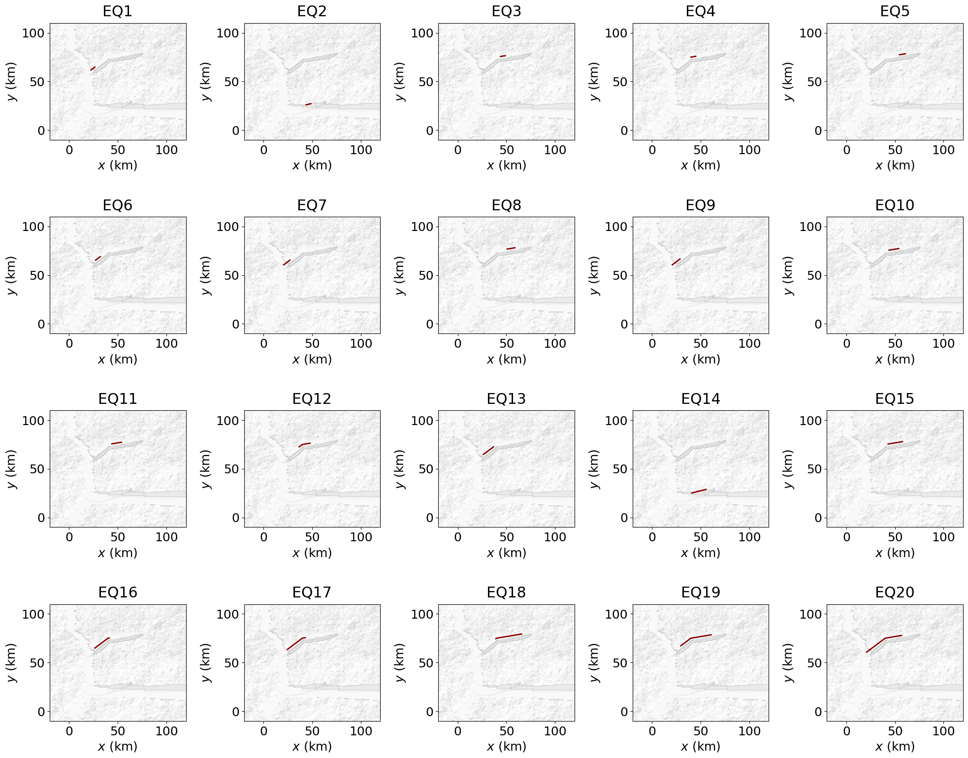
B.2. Earthquake case
The coordinates of stochastic events (defined in evchar) generally match those of their sources for localised peril sources (for diffuse sources, cellular automata are applied to determine the spatial characteristics of each event). In the case of earthquakes however, a floating rupture approach is used to generate earthquake ruptures on existing fault segments. The next cell illustrates how to extract the relevant information from evchar and how to examine the resulting spatial configuration in a stochastic run of EventSetGenerator().
EQcoord = evchar[GenMR_perils.get_peril_evID(evchar['evID']) == 'EQ'].reset_index(drop = True)
EQi = evtable[evtable['ID'] == 'EQ']['evID'].values

plt.rcParams['font.size'] = '18'
fig, ax = plt.subplots(4, 5, figsize=(20,16))
ax = ax.flatten()
for i in range(sizeDistr['EQ']['Nstoch']):
    EQcoord_evID = EQcoord[EQcoord['evID'] == EQi[i]]
    ax[i].contourf(grid.xx, grid.yy, GenMR_env.ls.hillshade(topoLayer.z, vert_exag=.1), cmap='gray', alpha = .1)
    ax[i].plot(EQcoord_evID['x'], EQcoord_evID['y'], color = 'darkred', linewidth = 2)
    ax[i].set_xlim(grid.xmin, grid.xmax)
    ax[i].set_ylim(grid.ymin, grid.ymax)
    ax[i].set_xlabel('$x$ (km)')
    ax[i].set_ylabel('$y$ (km)')
    ax[i].set_title(EQi[i], pad = 10)
    ax[i].set_aspect(1)
plt.tight_layout()
plt.pause(1)   # to avoid rare case where plot not displayed on notebook
plt.show()
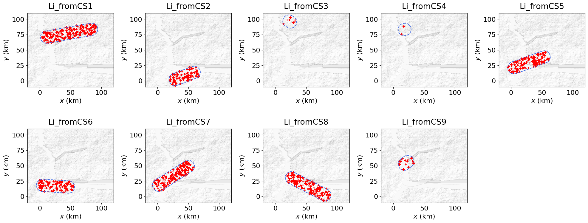
B.3. Lightning case
Lightning is triggered by convective storms. For a given CS* event, the corresponding Li_fromCS* event represents a set of lightning strikes, whose occurrence rate depends on the storm size (i.e., the cloud top height) and latitude. As shown below, lightning strikes are sampled from a spatially uniform random distribution within the storm footprint.
CS_coords = evchar[evchar['evID'].str[:2] == 'CS'].reset_index(drop = True)
Li_coords = evchar[evchar['evID'].str[:2] == 'Li'].reset_index(drop = True)
CS_list = CS_coords['evID'].unique()
Li_list = Li_coords['evID'].unique()

n_evID = len(CS_list)
max_cols = 5
ncols = min(n_evID, max_cols)
nrows = int(np.ceil(n_evID / ncols))

plt.rcParams['font.size'] = '16'
fig, ax = plt.subplots(nrows, ncols, figsize=(4 * ncols, 4 * nrows), squeeze=False)
ax = ax.flatten()
for i in range(n_evID):
    CS2plt = CS_coords[CS_coords['evID'] == CS_list[i]]
    Li2plt = Li_coords[Li_coords['evID'] == Li_list[i]]
    ax[i].contourf(grid.xx, grid.yy, GenMR_env.ls.hillshade(topoLayer.z, vert_exag=.1), cmap='gray', alpha = .1)
    ax[i].plot(CS2plt['x'], CS2plt['y'], color = GenMR_utils.col_peril('CS'), linestyle = 'dashed')
    ax[i].scatter(Li2plt['x'], Li2plt['y'], color = GenMR_utils.col_peril('Li'), marker = '+')
    ax[i].set_xlim(grid.xmin, grid.xmax)
    ax[i].set_ylim(grid.ymin, grid.ymax)
    ax[i].set_xlabel('$x$ (km)')
    ax[i].set_ylabel('$y$ (km)')
    ax[i].set_title(Li_list[i], pad = 10)
    ax[i].set_aspect(1)

for j in range(n_evID, len(ax)):
    ax[j].axis('off')

plt.tight_layout();
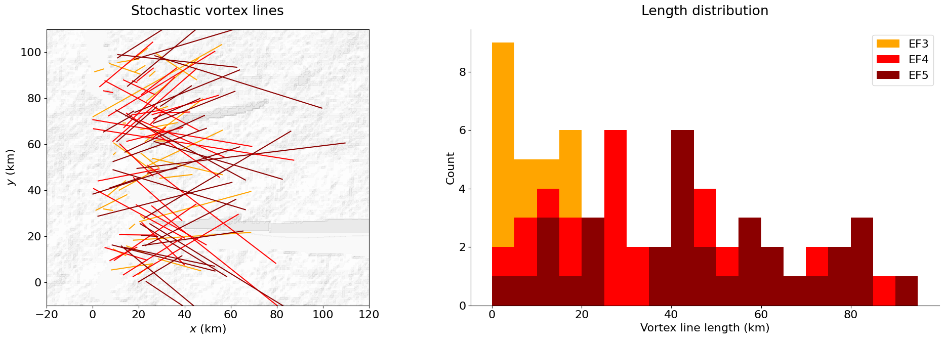
B.4. Tornado case
Change (e.g., increase) src_test.par['To']['N'] to test the stochastic properties of the tornado vortex-lines (i.e., initiation points random uniform, random strike, length according to EF-level Beta distribution).
TO IMPROVE: constrain initiation point locations (mask water mass and high altitude).
src_test = copy.deepcopy(src)
src_test.par['perils'] = ['To']
src_test.par['To']['N'] = 100
src_test.par['To']['theta_var'] = 45.
src_test.par['rdm_seed'] = None
sizeDistr_test = sizeDistr.copy()
sizeDistr_test['special'] = []     # remove 'CS'
sizeDistr_test['To']['Nstoch'] = src_test.par['To']['N']

eventSet_test = GenMR_perils.EventSetGenerator(src_test, sizeDistr_test, GenMR_utils)
evtable_test, evchar_test = eventSet_test.generate()

evchar_To = evchar_test[evchar_test['evID'].str.startswith('To')]
evIDi = evchar_To['evID'].unique()

L3 = np.array([])
L4 = np.array([])
L5 = np.array([])
plt.rcParams['font.size'] = '16'
fig, ax = plt.subplots(1,2, figsize = (20,7))
ax[0].contourf(grid.xx, grid.yy, GenMR_env.ls.hillshade(topoLayer.z, vert_exag=.1), cmap='gray', alpha = .1)
for i in evIDi:
    indev = evchar_To['evID'] == i
    x_To = evchar_To[indev]['x'].values
    y_To = evchar_To[indev]['y'].values
    L = np.sqrt((x_To[-1]-x_To[0])**2 + (y_To[-1]-y_To[0])**2)

    if evtable_test[evtable_test['evID'] == i]['S'].values == 3:
        col = 'orange'
        L3 = np.append(L3, L)
    elif evtable_test[evtable_test['evID'] == i]['S'].values == 4:
        col = 'red'
        L4 = np.append(L4, L)
    else:
        col = 'darkred'
        L5 = np.append(L5, L)
    ax[0].plot(x_To, y_To, color = col)

ax[0].set_xlim(grid.xmin, grid.xmax)
ax[0].set_ylim(grid.ymin, grid.ymax)
ax[0].set_xlabel('$x$ (km)')
ax[0].set_ylabel('$y$ (km)')
ax[0].set_title('Stochastic vortex lines', pad = 20)
ax[0].set_aspect(1)

bins = np.arange(0, src.par['To']['L_alpha_beta_Lmax_EF3'][2], 5)
ax[1].hist(L3, bins = bins, color = 'orange', label = 'EF3')
ax[1].hist(L4, bins = bins, color = 'red', label = 'EF4')
ax[1].hist(L5, bins = bins, color = 'darkred', label = 'EF5')
ax[1].set_xlabel('Vortex line length (km)')
ax[1].set_ylabel('Count')
ax[1].set_title('Length distribution', pad = 20)
ax[1].spines['right'].set_visible(False)
ax[1].spines['top'].set_visible(False)
ax[1].legend()

fig.tight_layout();
C. Hazard footprints
C.1. Tropical cyclone case
While modelling the AI, EQ, and VE intensity footprints from analytical expressions (Sect. 1.3.1) is straightforward, this is not the case for the TC peril, which involves a time-dependent intensity field. First, because the footprint depends on a moving track, a hazard-intensity field must be computed at each time increment, and the final static footprint is then defined as \(\max_t I(x,y,t)\). Second, the windfield is composed of several components, a tangential wind vector and the storm’s forward-motion vector, that must be combined to obtain the total wind amplitude. For illustration, intensity footprints at a given instant \(t\) are displayed below, together with their associated windfields, shown both without and with the effect of storm forward motion.
evID = 'TC5'     # choose a TC event
loc_x = 25.      # location of time snapshot (km)


track_evID = evchar[evchar['evID'] == evID]
t_snapshot = np.where(track_evID['x'] > loc_x)[0][0]

I_sym_t, I_asym_t, vtot_x, vtot_y, vtan_x, vtan_y = hazFootprints.get_TC_timeshot(evID, t_snapshot)


plt.rcParams['font.size'] = '18'
fig, ax = plt.subplots(1, 2, figsize=(20,10))

Imax = plot_Imax['TC']
I_plt = np.copy(I_sym_t)
I_plt[I_plt >= Imax] = Imax
ax[0].contourf(grid.xx, grid.yy, I_plt, cmap = 'Reds', levels = np.linspace(0, Imax, 100), vmin=33, vmax=Imax)
ax[0].plot(track_evID['x'], track_evID['y'], color = GenMR_utils.col_peril('TC'))
ax[0].plot(src.SS_char['x'], src.SS_char['y'], color = 'black', linestyle = 'dashed')
ax[0].scatter(track_evID['x'].values[t_snapshot], track_evID['y'].values[t_snapshot], marker = '+', \
              color = 'black', s = 200)
delta = 50
for i in range(int(grid.xx.shape[0]/delta)):
    for j in range(int(grid.xx.shape[1]/delta)):
        ax[0].arrow(grid.xx[delta*i,delta*j], grid.yy[delta*i,delta*j],
            .05 * vtan_x[delta*i,delta*j], .05* vtan_y[delta*i,delta*j], head_width = 1, color = 'white')
ax[0].set_xlabel('$x$ (km)')
ax[0].set_ylabel('$y$ (km)')
ax[0].set_title('Static storm', pad = 20)
ax[0].set_xlim(grid.xmin, grid.xmax)
ax[0].set_ylim(grid.ymin, grid.ymax)
ax[0].set_aspect(1)

I_plt = np.copy(I_asym_t)
I_plt[I_plt >= Imax] = Imax
ax[1].contourf(grid.xx, grid.yy, I_plt, cmap = 'Reds', levels = np.linspace(0, Imax, 100), vmin=33, vmax=Imax)
ax[1].plot(track_evID['x'], track_evID['y'], color = GenMR_utils.col_peril('TC'))
ax[1].plot(src.SS_char['x'], src.SS_char['y'], color = 'black', linestyle = 'dashed')
ax[1].scatter(track_evID['x'].values[t_snapshot], track_evID['y'].values[t_snapshot], marker = '+', \
              color = 'black', s = 200)
delta = 50
for i in range(int(grid.xx.shape[0]/delta)):
    for j in range(int(grid.xx.shape[1]/delta)):
        ax[1].arrow(grid.xx[delta*i,delta*j], grid.yy[delta*i,delta*j],
            .05 * vtot_x[delta*i,delta*j], .05* vtot_y[delta*i,delta*j], head_width = 1, color = 'white')
ax[1].set_xlabel('$x$ (km)')
ax[1].set_ylabel('$y$ (km)')
ax[1].set_title('Storm in motion', pad = 20)
ax[1].set_xlim(grid.xmin, grid.xmax)
ax[1].set_ylim(grid.ymin, grid.ymax)
ax[1].set_aspect(1)
plt.tight_layout();
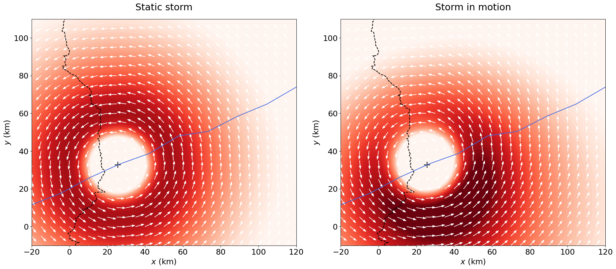
C.2. Tornado case
Since tornado intensity footprints appear as linear features at the digital template scale, the following cell zooms into a segment of a maximum wind-speed footprint to illustrate the lateral asymmetry of the wind field perpendicular to the source line.
evID = 'To1'

To_coord = evchar[evchar['evID'] == evID].reset_index(drop=True)
vmax = catalog_hazFootprints[evID]
# add signed lateral distance
r2To = GenMR_perils.HazardFootprintGenerator.calc_lateral_distance_signed(grid.xx, grid.yy, To_coord['x'], To_coord['y'])


plt.rcParams['font.size'] = '18'
fig, ax = plt.subplots(1,3, figsize = (20,7))
ax[0].contourf(grid.xx, grid.yy, r2To, cmap = 'seismic', vmin = -50, vmax = 50, levels = np.linspace(-100, 100, 201))
ax[0].contourf(grid.xx, grid.yy, GenMR_env.ls.hillshade(topoLayer.z, vert_exag=.1), cmap='gray', alpha = .1)
dx = To_coord['x'].values[-1] - To_coord['x'].values[0]
dy = To_coord['y'].values[-1] - To_coord['y'].values[0]
ax[0].arrow(To_coord['x'][0], To_coord['y'][0], dx, dy, color = 'black', head_width = 5)
ax[0].set_xlim(grid.xmin, grid.xmax)
ax[0].set_ylim(grid.ymin, grid.ymax)
ax[0].set_xlabel('$x$ (km)')
ax[0].set_ylabel('$y$ (km)')
ax[0].set_title('Signed lateral dist. to path')
ax[0].set_aspect(1)

ax[1].contourf(grid.xx, grid.yy, vmax, cmap = 'Reds', vmin = 40, vmax = 80)
ax[1].contourf(grid.xx, grid.yy, GenMR_env.ls.hillshade(topoLayer.z, vert_exag=.1), cmap='gray', alpha = .1)
ax[1].set_xlim(grid.xmin, grid.xmax)
ax[1].set_ylim(grid.ymin, grid.ymax)
ax[1].set_xlabel('$x$ (km)')
ax[1].set_ylabel('$y$ (km)')
ax[1].set_title(f'{evID} footprint')
ax[1].set_aspect(1)

To_x0, To_y0 = To_coord['x'].mean(), To_coord['y'].mean()
dxy = 1.  # km on each side of (x0,y0)
ax[2].contourf(grid.xx, grid.yy, vmax, cmap = 'Reds', vmin = 40, vmax = 80)
ax[2].contourf(grid.xx, grid.yy, GenMR_env.ls.hillshade(topoLayer.z, vert_exag=.1), cmap='gray', alpha = .1)
ax[2].plot(To_coord['x'], To_coord['y'], color = 'white', linestyle = 'dotted')
ax[2].set_xlim(To_x0-dxy, To_x0+dxy)
ax[2].set_ylim(To_y0-dxy, To_y0+dxy)
ax[2].set_xlabel('$x$ (km)')
ax[2].set_ylabel('$y$ (km)')
ax[2].set_title(f'{evID} footprint zoomed in')
ax[2].set_aspect(1);
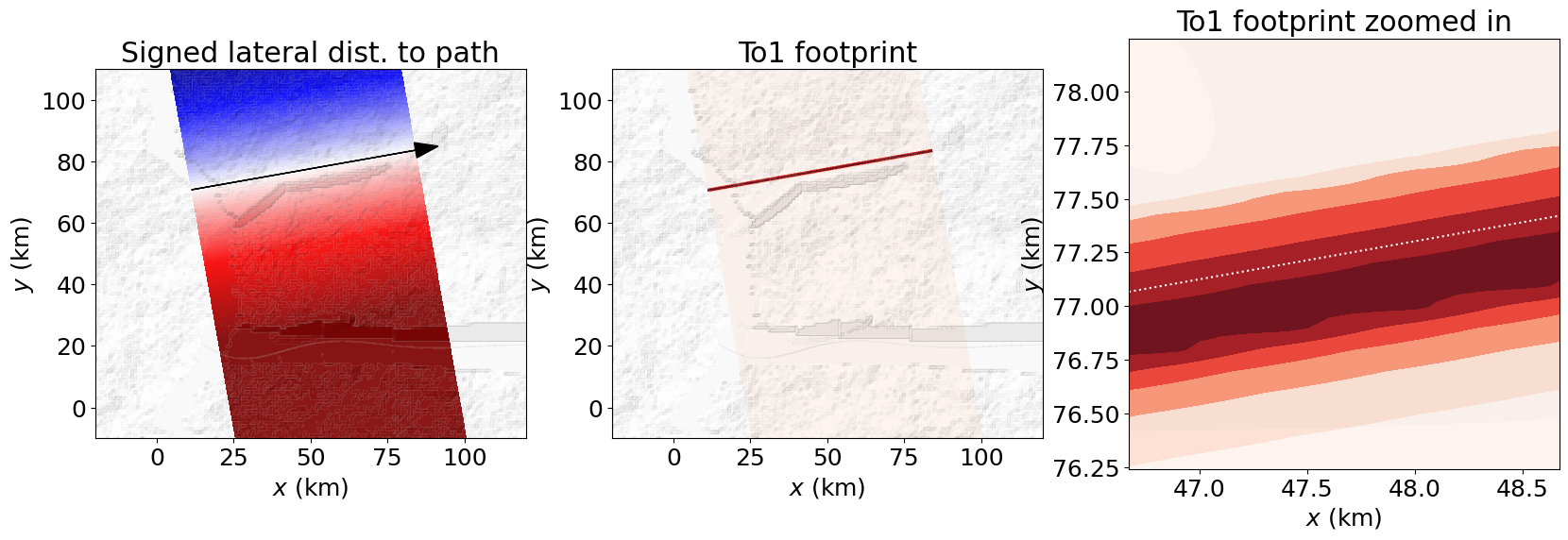
C.3. Heatwave case (threshold model)
Heatwave HW temperature footprints are generated using a threshold-based model, in which an event is declared when the temperature equals or exceeds T_th for at least Dt_da consecutive days. Temperature extremes in the digital template arise from the combination of large-scale advective temperature anomalies and temporally correlated daily temperature variability.
The parameter nsig can be adjusted to explore different levels of heatwave extremity within the digital template.
NOTE: Tadv (synoptic advective regime) is drawn once per simulation, hence held constant over the 4-week window considered (with Dt_max_da = 30). This is a deliberate simplification of a regime-switching (semi-Markov) advection process, justified as follows: (i) synoptic advective regimes (persistent warm/cold air-mass intrusions) typically persist on the order of 1–4 weeks, consistent with a monthly-block approximation; (ii) it reproduces the skewed, heavy-tailed character of advective bursts responsible for heatwave onset, which the unimodal AR(1) alone cannot capture. See Tutorial 3 for the full-year treatment, where Tadv is sampled as a regime-switching (semi-Markov) process over the full simulation period rather than fixed to a single 30-day window.
from scipy.stats import norm

nsig = 3                                       # mean temperature extreme observed at nsigma
rdm_seed = 4                                   # None or integer - to test different daily fluctuations
Tmin, Tmax = 10, 40                            # range considered
month = 7

T_th = src.par['HW']['T_th']
Dt = src.par['HW']['Dt_da']
sigmaT_yearly =src.par['HW']['sigmaT_yearly']
Ndays = src.par['HW']['Dt_max_da']
dayi = np.arange(src.par['HW']['Dt_max_da'])+1
lat = grid.par['lat_deg']

Ti = np.arange(Tmin, Tmax, 1)
T0 = np.max(atmoLayer.T)                       # digital template near-surface air temperature f(lat, month)
Tnorm_pdf = norm.pdf(Ti, T0, sigmaT_yearly)    # annual variations of mean temperature

# advection model (3-Gaussian model)
Tadv_pdf, Tadv_sigma, advection_comp = GenMR_perils.HazardFootprintGenerator.pdf_T_advectivemodel(Ti, T0, lat)

Tadv_nsig = T0 + nsig * Tadv_sigma             # nsigma advective event
                                               # note: the stochastic version also includes sigmaT_yearly role
# temperature daily variations over Ndays
T_plt = Tadv_nsig   # close enough to HW threshold to observe HW periods
Tdaily_stoch_plt = GenMR_perils.HazardFootprintGenerator.sample_T_AR1process(T_plt, Ndays, \
                        src.par['HW']['T_AR1'][0], src.par['HW']['T_AR1'][1], seed = rdm_seed)

# for illustration: extract heatwave events according to time series only
HW_ti_plt, HW_Dt_plt = GenMR_perils.HazardFootprintGenerator.get_HW_atloc(Tdaily_stoch_plt, T_th, Dt)


# define HW footprint
DTadv_nsig = Tadv_nsig - T0                          # advection shift
Tmap_mean = atmoLayer.T[month-1,:,:] + DTadv_nsig    # mean temp. map of the nsigma day, before daily fluctuations
DTdaily_stoch = Tdaily_stoch_plt - Tadv_nsig         # daily fluctuations

nx, ny = Tmap_mean.shape
Tmap_daily_stoch = np.empty((Ndays, nx, ny))
for t in range(Ndays):
     Tmap_daily_stoch[t] = Tmap_mean + DTdaily_stoch[t]
HW_fp, HW_S = GenMR_perils.HazardFootprintGenerator.get_HW_footprint(Tmap_daily_stoch, Tth=T_th, Dt=Dt)


plt.rcParams['font.size'] = '16'
fig, ax = plt.subplots(2,4, figsize=(20,10))

ax[0,0].contourf(grid.xx, grid.yy, GenMR_env.ls.hillshade(topoLayer.z, vert_exag=.1), cmap='gray')
img = ax[0,0].contourf(grid.xx, grid.yy, atmoLayer.T[month-1,:,:], cmap = 'bwr', vmin=0, vmax=30, alpha = .5)
ax[0,0].set_xlabel('$x$ (km)')
ax[0,0].set_ylabel('$y$ (km)')
ax[0,0].set_title('Average temperature', pad = 20)
ax[0,0].set_aspect(1)
fig.colorbar(img, ax = ax[0,0], fraction = .04, pad = .04, label = 'Temperature (°C)')

ax[0,1].contourf(grid.xx, grid.yy, GenMR_env.ls.hillshade(topoLayer.z, vert_exag=.1), cmap='gray')
img = ax[0,1].contourf(grid.xx, grid.yy, atmoLayer.T[month-1,:,:] + nsig * Tadv_sigma, cmap = 'bwr', \
                 vmin=0, vmax=30, alpha = .5)
ax[0,1].set_xlabel('$x$ (km)')
ax[0,1].set_ylabel('$y$ (km)')
ax[0,1].set_title(f'Advection temp. at {nsig}$\sigma$', pad = 20)
ax[0,1].set_aspect(1)
fig.colorbar(img, ax = ax[0,1], fraction = .04, pad = .04, label = 'Temperature (°C)')

ax[0,2].contourf(grid.xx, grid.yy, GenMR_env.ls.hillshade(topoLayer.z, vert_exag=.1), cmap='gray')
img = ax[0,2].contourf(grid.xx, grid.yy, atmoLayer.T[month-1,:,:] + DTadv_nsig + np.max(DTdaily_stoch), \
                       cmap = 'bwr', vmin=0, vmax=30, alpha = .5)
ax[0,2].set_xlabel('$x$ (km)')
ax[0,2].set_ylabel('$y$ (km)')
ax[0,2].set_title(f'Max. daily temp. at {nsig}$\sigma$', pad = 20)
ax[0,2].set_aspect(1)
fig.colorbar(img, ax = ax[0,2], fraction = .04, pad = .04, label = 'Temperature (°C)')

ax[0,3].axis('off')


ax[1,0].plot(Ti, Tnorm_pdf, color='black')
ax[1,0].axvline(T0, color = 'black', linestyle = 'dashed', label = '$T_0$')
ax[1,0].axvline(T0 + nsig * sigmaT_yearly, color = 'black', linestyle = 'dotted', label = f'$T_0+{nsig}\sigma$')
ax[1,0].axvline(T_th, color = 'darkred', linestyle = 'dashed', label = '$T_{th}$')
ax[1,0].set_xlabel('$T$ (°C)')
ax[1,0].set_ylabel('Density')
ax[1,0].set_title('Baseline', pad = 20)
ax[1,0].spines['right'].set_visible(False)
ax[1,0].spines['top'].set_visible(False)
ax[1,0].legend(fontsize = 12)

ax[1,1].plot(Ti, advection_comp['pdf0'], color='green', linestyle = 'dashed', label = 'baseline')
ax[1,1].plot(Ti, advection_comp['pdf_c'], color='blue', linestyle = 'dashed', label = 'cold flux')
ax[1,1].plot(Ti, advection_comp['pdf_w'], color='red', linestyle = 'dashed', label = 'warm flux')
ax[1,1].plot(Ti, Tadv_pdf, color='black')
ax[1,1].axvline(T0, color = 'black', linestyle = 'dashed')
ax[1,1].axvline(Tadv_nsig, color = 'black', linestyle = 'dotted')
ax[1,1].axvline(T_th, color = 'darkred', linestyle = 'dashed')
ax[1,1].set_xlabel('$T$ (°C)')
ax[1,1].set_ylabel('Density')
ax[1,1].set_title('Advection', pad = 20)
ax[1,1].spines['right'].set_visible(False)
ax[1,1].spines['top'].set_visible(False)
ax[1,1].legend(fontsize = 12)

dayi = np.arange(Ndays)+1
ax[1,2].plot(dayi, Tdaily_stoch_plt, color = 'black')
for start, end in HW_ti_plt:
    ax[1,2].axvspan(dayi[start] - .5, dayi[end] + .5, color='darkred', alpha = .2)
ax[1,2].axhline(T_plt, color = 'black', linestyle = 'dotted')
ax[1,2].axhline(T_th, color = 'darkred', linestyle = 'dashed')
ax[1,2].set_ylim(T_th-5, T_th+5)
ax[1,2].set_xlabel('Day of the month')
ax[1,2].set_ylabel('$T$ (°C)')
ax[1,2].set_title(f'Daily temp. at +{nsig}$\sigma$={Tadv_nsig:.1f}°C', pad = 20)
ax[1,2].spines['right'].set_visible(False)
ax[1,2].spines['top'].set_visible(False)

ax[1,3].contourf(grid.xx, grid.yy, GenMR_env.ls.hillshade(topoLayer.z, vert_exag=.1), cmap='gray')
ax[1,3].contourf(grid.xx, grid.yy, HW_fp, cmap = 'Reds', alpha = .5)
ax[1,3].set_xlabel('$x$ (km)')
ax[1,3].set_ylabel('$y$ (km)')
ax[1,3].set_title(f'{nsig}$\sigma$ heatwave fp. ({HW_S} da)', pad = 20)
ax[1,3].set_aspect(1)

plt.tight_layout();
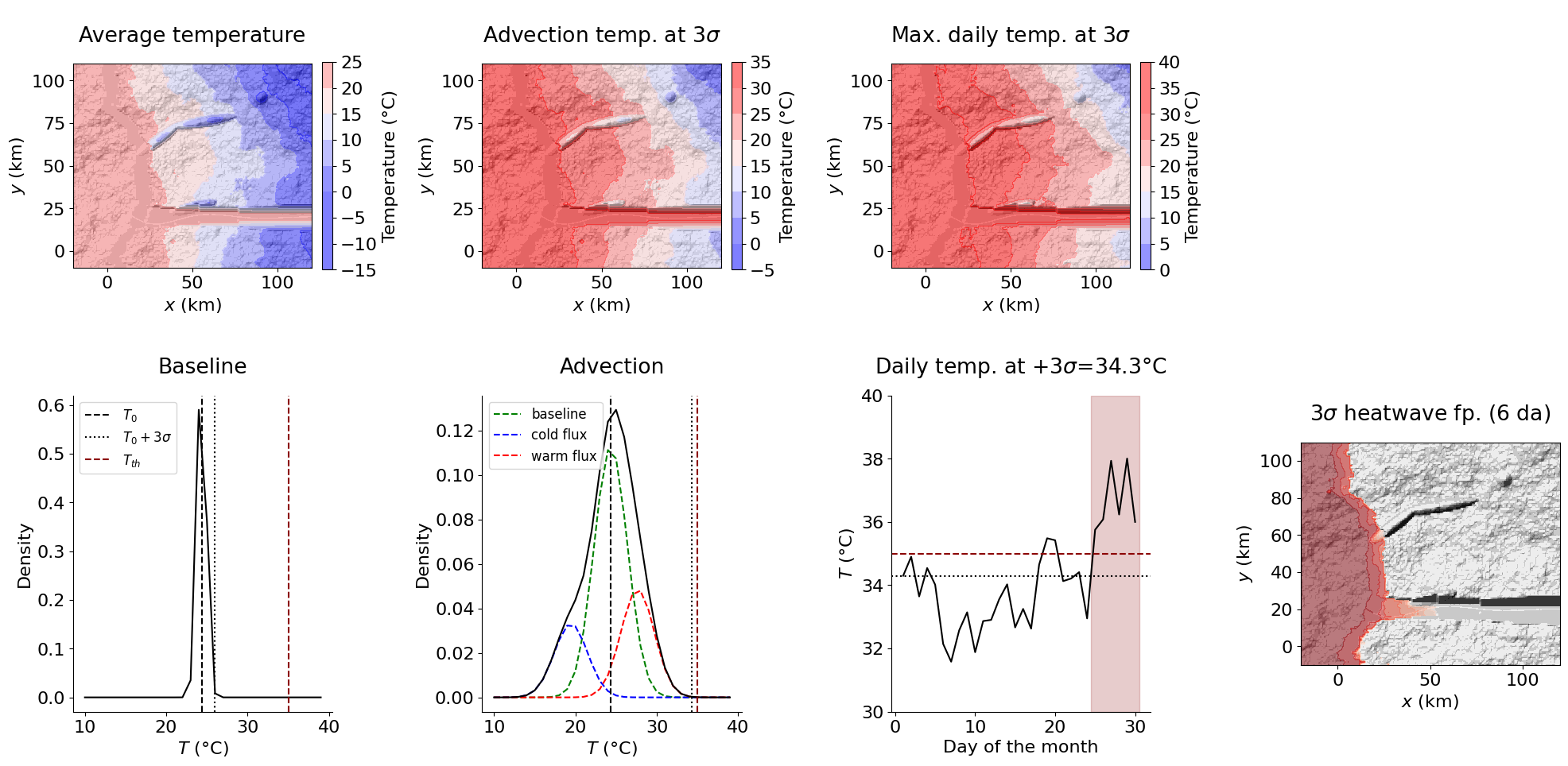
C.4. Pest infestation case
Pest infestation (PI) intensity is modelled analytically. Based on the temperature-dependent development rate of the pest (here Spodoptera frugiperda, see calc_PI_growthrate()), the hazard intensity is defined as a unitless index representing the expected number of pest larvae after one month (on the fixed time scale considered in Tutorial 2), normalised by the corresponding number at the optimal growth temperature \(T_{opt}\) (see calc_PI_I()). Consequently, at the optimal temperature the intensity equals 1, corresponding to 100% yield loss for crops located at \(T(x,y) = T_{opt}\). The resulting footprint is defined only over crop locations.
DTadv = 15    # change this value to explore impact of high temperatures relative to average temperature for July
              # DTadv represents the temperature increase from advection during heat wave


Ti = np.arange(0, 50, .1)
growrate_pest_i = GenMR_perils.HazardFootprintGenerator.calc_PI_growthrate(Ti, 'Shi')  # see other models in func.
haz_index_i, Topt = GenMR_perils.HazardFootprintGenerator.calc_PI_I(Ti, 'Shi')

month = 7
T_map = atmoLayer.T[month-1,:,:] + DTadv
haz_index_map, _ = GenMR_perils.HazardFootprintGenerator.calc_PI_I(T_map, 'Shi')
mask_crop = urbLandLayer.S >= 5

PI_fp = haz_index_map * mask_crop.astype(int)
PI_fp[PI_fp == 0] = np.nan

plt.rcParams['font.size'] = '16'
fig, ax = plt.subplots(1,3, figsize=(20,6))

ax[0].plot(Ti, growrate_pest_i, color = 'black')
ax[0].set_xlabel('$T$ (°C)')
ax[0].set_ylabel('Growth rate (/day)')
ax[0].set_title('Pest growth function', pad = 20)
ax[0].legend()
ax[0].spines['right'].set_visible(False)
ax[0].spines['top'].set_visible(False)

ax[1].plot(Ti, haz_index_i, color = 'black', label = 'hazard index')
ax[1].axvline(Topt, color = 'black', linestyle = 'dotted', label = "pest's $T_{opt}$")
ax[1].axvline(np.max(T_map), color = 'black', linestyle = 'dashed', label = "region's max. $T$")
ax[1].set_xlabel('$T$ (°C)')
ax[1].set_ylabel('Severity index (yield loss ratio)')
ax[1].set_title('Pest severity', pad = 20)
ax[1].legend()
ax[1].spines['right'].set_visible(False)
ax[1].spines['top'].set_visible(False)

S_map = int(np.nanmean(PI_fp) * 100)

ax[2].contourf(grid.xx, grid.yy, GenMR_env.ls.hillshade(topoLayer.z, vert_exag=.1), cmap='gray')
ax[2].contourf(grid.xx, grid.yy, PI_fp, cmap = 'Reds', vmin=0, vmax=1, alpha = .5)
ax[2].set_xlabel('$x$ (km)')
ax[2].set_ylabel('$y$ (km)')
ax[2].set_title(f'PI footprint: mean yield reduction = {S_map}%', pad = 20)
ax[2].set_aspect(1)

plt.tight_layout();
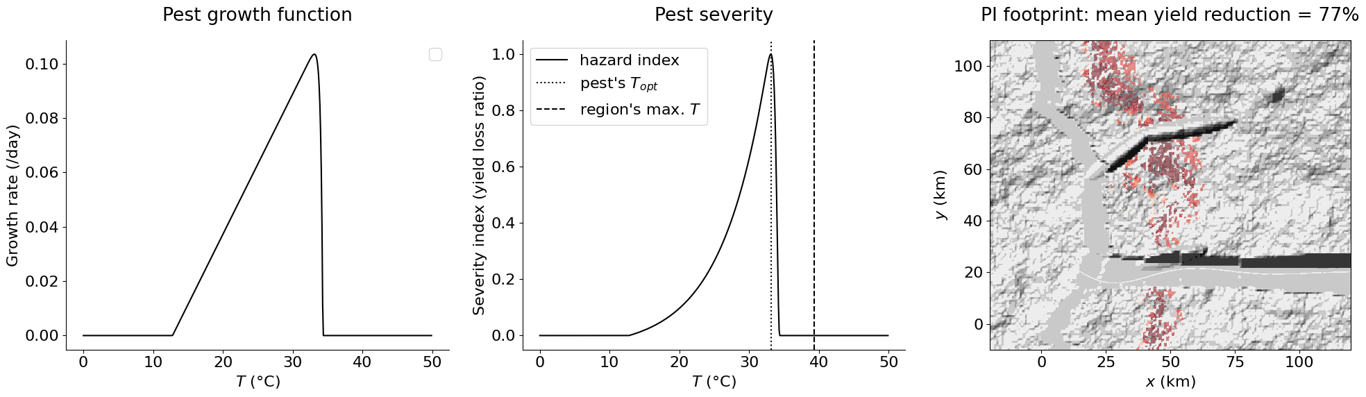
C.5. Blackout case
Since blackouts (BO) are an invisible secondary peril, they do not enter the simple hazard-to-damage footprint process developed in this tutorial. The model is therefore demonstrated in this appendix for various damage scenarios and will be appied in Tutorial 3 where damage to the power grid will be due by other perils. Consequences are business interruption and public service failure (see Sections C.6 and C.7).
## SCENARIO ##
period = 'day'                       # 'day' or 'night'
src.par['BO']['tolerance'] = 1       # high value to correct simplified topology (more redundancies in reality)
                                     # and lack of protection systems present in reality
                                     # value of 2 from trial and error, rare cascades when 1 element removed


# see map with node names to select which elements fail. Map created using:
# GenMR_env.plot_EnvLayer_attr(energyLayer, 'powergrid_wID', file_ext = 'pdf') & zoom on pdf file if needed
failed_nodes = []
#failed_nodes = ['Gdam_1', 'Gdam_2', 'Gdam_3', 'Gth_1', 'Gth_2', 'Gth_3', 'Gwf_1', 'Gwf_2', 'Gwf_3'] # zero power
#failed_nodes = ['Gdam_1', 'Gdam_2', 'Gdam_3']
#failed_nodes = ['Gth_1', 'Gth_2', 'Gth_3']
#failed_nodes = ['Gwf_1', 'Gwf_2', 'Gwf_3']
#failed_nodes = ['L8']
#failed_nodes = ['L17']
#failed_nodes = ['L35']
failed_lines = []
#failed_lines = [('T111', 'T112'), ('T165', 'T166'), ('T140', 'T141')]
#failed_lines = [('T165', 'T166'), ('T140', 'T141')]
#failed_lines = [('T140', 'T141')]
failed_lines = [('L33', 'L35')]   # ***
#failed_lines = [('L13', 'L19')]
#failed_lines = [('L16', 'L22')]
#failed_lines = [('L5', 'L6'), ('L2', 'L6')]
##############


powergrid_g, node_names, node_coords, node_supply = energyLayer.powergrid
node_names_list = [node_names[i] for i in range(len(node_names))]
indL = [i for i, name in node_names.items() if name.startswith('L')]
indS = [i for i, name in node_names.items() if name.startswith('S')]
indG = [i for i, name in node_names.items() if name.startswith('G')]
node_coords = np.array(node_coords)
L_coords = node_coords[indL]
S_coords = node_coords[indS]
G_coords = node_coords[indG]
edges = list(powergrid_g.edges())
slack_id = next(i for i, name in node_names.items() if name.startswith('Gdam'))

if period == 'day':
    node_served = energyLayer.node_served_day
    node_demand = energyLayer.node_demand_served_day
#    node_demand = socioecoLayer.node_demand_day
else:
    node_served = energyLayer.node_served_night
    node_demand = energyLayer.node_demand_served_night
#    node_demand = socioecoLayer.node_demand_night


BO_loads, g_BO, g_dmg, g_intact, node_served_BO, node_supply_dmg = GenMR_perils.run_BO_flow(energyLayer,
                                                  src.par['BO'], \
                                                  failed_nodes, failed_lines, slack_id = slack_id, \
                                                  period = period, print_casc = True)


n_nodes = len(node_names)
A_dmg = GenMR_utils.graph_to_full_adjacency(g_dmg, n_nodes)
A_BO  = GenMR_utils.graph_to_full_adjacency(g_BO,  n_nodes)
print('Operational grid - Power supply (MW) per load node:\n', node_served[indL])
print('Load nodes offline during blackout:\n', BO_loads)
print('During blackout - Power supply (MW) per load node:\n', node_served_BO[indL])


plt.rcParams['font.size'] = 16
fig, ax = plt.subplots(2, 2, figsize=(20, 14))

s_node, s_maxsupply, s_BO = 20, 200, 500
eps = 5
xmin_BO, xmax_BO = node_coords[:, 0].min() - eps, node_coords[:, 0].max() + eps
ymin_BO, ymax_BO = node_coords[:, 1].min() - eps, node_coords[:, 1].max() + eps


## physical power grid ##
ax[0,0].contourf(grid.xx, grid.yy, GenMR_env.ls.hillshade(topoLayer.z, vert_exag=.1), cmap='gray', alpha = .1)
ax[0,0].scatter(L_coords[:,0], L_coords[:,1], color='black', s=s_node, label='Load')
ax[0,0].plot(S_coords[:,0], S_coords[:,1], 'bs', markersize=s_node, label='Substation')
ax[0,0].plot(G_coords[:,0], G_coords[:,1], 'r*', markersize=s_node, label='Generator')
for ii,jj in edges:
    x = [node_coords[ii,0], node_coords[jj,0]]
    y = [node_coords[ii,1], node_coords[jj,1]]
    ax[0,0].plot(x, y, color='black', linewidth=0.5)
ax[0,0].set_xlabel('$x$ (km)')
ax[0,0].set_ylabel('$y$ (km)')
ax[0,0].set_title('Physical power grid', pad = 20)
ax[0,0].set_aspect(1)
ax[0,0].legend(loc='upper right')
ax[0,0].set_xlim(xmin_BO, xmax_BO)
ax[0,0].set_ylim(ymin_BO, ymax_BO)


## Operational power grid ##
scale_factor = s_maxsupply / node_served[indL].max()
load_sizes = node_served[indL] * scale_factor

#node_demand_full = np.zeros(n_nodes)
#node_demand_full[indL] = node_demand
flows_op = energyLayer._compute_flows_dc(powergrid_g, node_supply, node_demand, slack_id = slack_id)[0]
edge_width_op = []
for i, j in edges:
    f = abs(flows_op.get((i,j), flows_op.get((j,i), 0.0)))
    # scale for plotting, max width = 10
    edge_width_op.append(1 + 9*f/np.max(list(flows_op.values())))

ax[0,1].contourf(grid.xx, grid.yy, GenMR_env.ls.hillshade(topoLayer.z, vert_exag=.1), cmap = 'gray', alpha = .1)
for (i,j), w in zip(edges, edge_width_op):
    ax[0,1].plot([node_coords[i,0], node_coords[j,0]],
                 [node_coords[i,1], node_coords[j,1]],
                 color='green', linewidth=w)
ax[0,1].scatter(L_coords[:,0], L_coords[:,1], color='green', s=load_sizes)
for i, (x, y) in enumerate(node_coords):
    ax[0,1].text(x + 1, y + 1, node_names[i], fontsize=8, zorder=3)
ax[0,1].set_xlabel('$x$ (km)')
ax[0,1].set_ylabel('$y$ (km)')
ax[0,1].set_title(f'Operational power grid during {period}', pad=20)
ax[0,1].set_aspect(1)
ax[0,1].set_xlim(xmin_BO, xmax_BO)
ax[0,1].set_ylim(ymin_BO, ymax_BO)


## Damaged grid ##
edge_col_dmg = np.array(['grey' if A_dmg[i,j]==1 else 'red' for i,j in edges])
edge_lw_dmg = np.array([1 if A_dmg[i,j]==1 else 5 for i,j in edges])
node_col_dmg = np.array(['red' if node_names[i] in failed_nodes else 'grey' for i in range(n_nodes)])
node_s_dmg = np.array([10*s_node if node_names[i] in failed_nodes else s_node for i in range(n_nodes)])

ax[1,0].contourf(grid.xx, grid.yy, GenMR_env.ls.hillshade(topoLayer.z, vert_exag=.1),
                 cmap='gray', alpha=0.1)
for (i,j), color, lw in zip(edges, edge_col_dmg, edge_lw_dmg):
    x = [node_coords[i,0], node_coords[j,0]]
    y = [node_coords[i,1], node_coords[j,1]]
    ax[1,0].plot(x, y, color=color, linewidth=lw)
ax[1,0].scatter(node_coords[:,0], node_coords[:,1], color=node_col_dmg, s=node_s_dmg, zorder=2)
ax[1,0].set_xlabel('$x$ (km)')
ax[1,0].set_ylabel('$y$ (km)')
ax[1,0].set_title('Exogenic damage', pad=20)
ax[1,0].set_aspect(1)
ax[1,0].legend(loc='upper right')
ax[1,0].set_xlim(xmin_BO, xmax_BO)
ax[1,0].set_ylim(ymin_BO, ymax_BO)


## Blackout footprint ##
fraction_acceptable = .1   # if loss greater than 10%, shown in orange = brownout / partial supply
fraction_served = (node_served_BO[indL] - node_demand[indL])/node_demand[indL]

load_nodes = [node_names[i] for i in indL]
load_col_BO = np.array([
    'black' if name in BO_loads else
    'darkorange' if fraction_served[i] < -fraction_acceptable else
    'green'
    for i, name in enumerate(load_nodes)
])
load_s_BO = scale_factor * node_served_BO[indL]
load_s_BO = np.array([s_BO if name in BO_loads else load_s_BO[i] for i, name in enumerate(load_nodes)])

edge_col_BO = []
for i, j in edges:
    in_BO  = (i, j) in g_BO.edges()  or (j, i) in g_BO.edges()
    in_dmg = (i, j) in g_dmg.edges() or (j, i) in g_dmg.edges()

    if not in_dmg:    # physically destroyed
        edge_col_BO.append('red')
    elif not in_BO:   # tripped during cascade
        edge_col_BO.append('darkred')
    else:
        edge_col_BO.append('green')

#node_supply_dmg = node_supply.copy().astype(float)
#for name in failed_nodes:
#    idx = node_names_list.index(name)
#    node_supply_dmg[idx] = 0.          # zero generator supply if applicable

flows_BO = energyLayer._compute_flows_dc(g_BO, node_supply_dmg, node_demand, slack_id = slack_id)[0]
edge_width_BO = []
for i, j in edges:
    f = abs(flows_BO.get((i,j), flows_BO.get((j,i), 0.0)))
    # scale for plotting, max width = 10
    edge_width_BO.append(1 + 9*f/np.max(list(flows_op.values())))

ax[1,1].contourf(grid.xx, grid.yy, GenMR_env.ls.hillshade(topoLayer.z, vert_exag=.1),
                 cmap='gray', alpha=0.1)
for (i,j), color, w in zip(edges, edge_col_BO, edge_width_BO):
    x = [node_coords[i,0], node_coords[j,0]]
    y = [node_coords[i,1], node_coords[j,1]]
    ax[1,1].plot(x, y, color=color, linewidth=w)

for i, c, s in zip(indL, load_col_BO, load_s_BO):
    ax[1,1].scatter(node_coords[i,0], node_coords[i,1], color=c, s=s, zorder=2)
ax[1,1].set_xlabel('$x$ (km)')
ax[1,1].set_ylabel('$y$ (km)')
ax[1,1].set_title(f'Blackout footprint during {period}', pad=20)
ax[1,1].set_aspect(1)
ax[1,1].set_xlim(xmin_BO, xmax_BO)
ax[1,1].set_ylim(ymin_BO, ymax_BO)

plt.tight_layout();
[step 0] overloaded edges: 10 / 252
[cascade] step 1, failing edges: [(8, np.int64(12)), (9, np.int64(10)), (9, np.int64(15)), (11, np.int64(12)), (11, np.int64(17)), (12, np.int64(18)), (18, np.int64(19)), (24, np.int64(25)), (25, np.int64(28)), (28, np.int64(32))]
[cascade] no more overloads — stopped after 1 step(s).
Operational grid - Power supply (MW) per load node:
 [249.25382068 244.92499118 113.77183873 181.15234868 227.25538901
 147.31680893 142.29796826 154.28320645 102.04749    288.24408734
 114.73491526 204.5314592  137.74974547 168.4450112   84.57843787
 479.36494695  93.08021596 135.16738026 112.45537136 109.28500391
  53.42251121 405.0518215  164.11417477 101.10820031 105.78730767
  72.21580947 392.02166719 141.50955194 154.09336249  32.28974321
 482.26015867 118.52968641  81.0198384  239.79748706 187.55026817
 166.19700609  58.74738686 276.82288953  92.11370765  52.32794301
  24.18836862]
Load nodes offline during blackout:
 ['L35', 'L37', 'L39', 'L40', 'L41']
During blackout - Power supply (MW) per load node:
 [249.25382068 244.92499118 113.77183873 181.15234868 227.25538901
 147.31680893 142.29796826 154.28320645 102.04749    288.24408734
 114.73491526 204.5314592  137.74974547 168.4450112   84.57843787
 479.36494695  93.08021596 135.16738026 112.45537136 109.28500391
  53.42251121 405.0518215  164.11417477 101.10820031 105.78730767
  72.21580947 392.02166719 141.50955194 154.09336249  32.28974321
 482.26015867 118.52968641  81.0198384  239.79748706   0.
 166.19700609   0.         276.82288953   0.           0.
   0.        ]
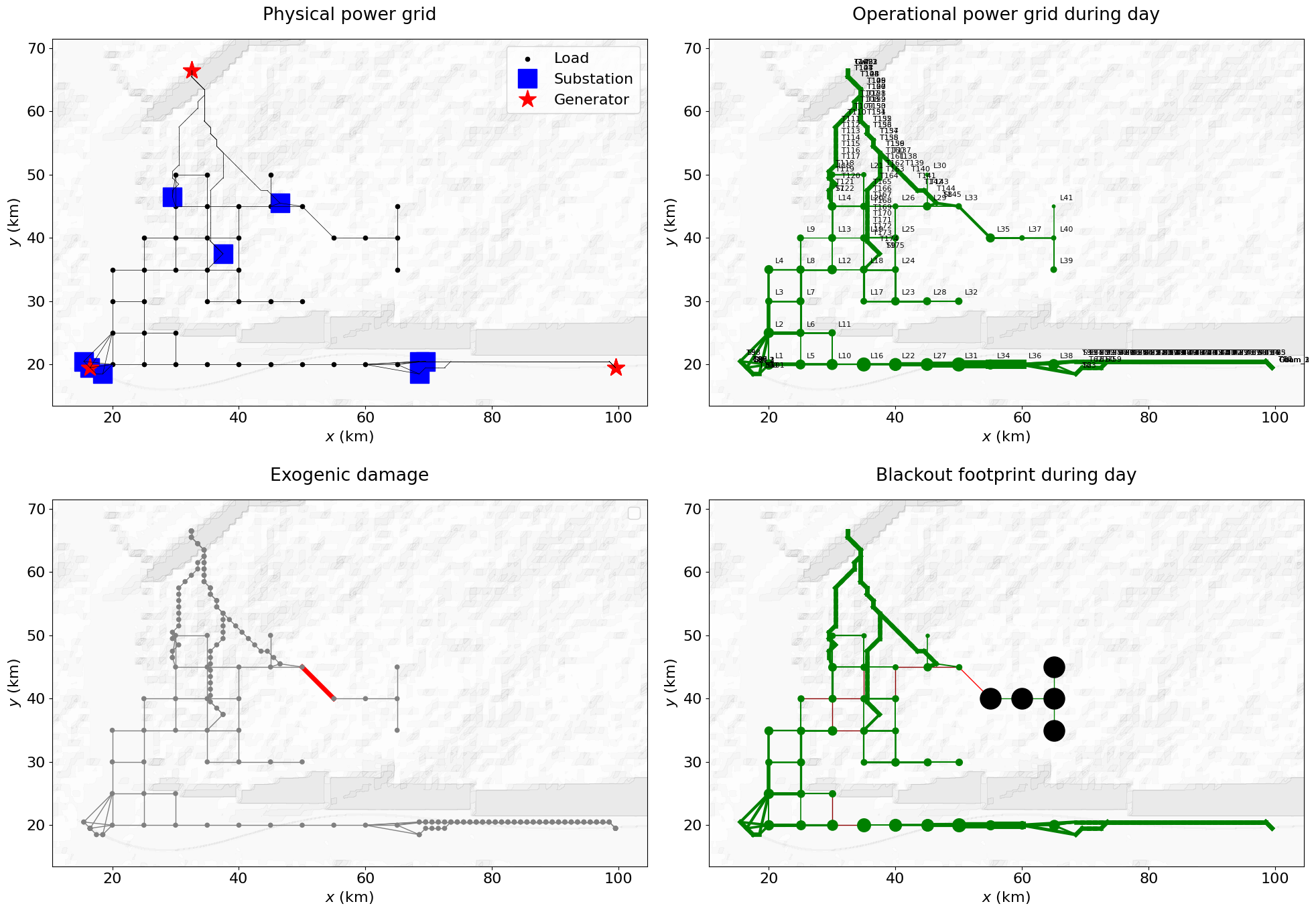
C.6. Business interruption case
Similarly to BO, BI will be studied in detail in Tutorial 3 in the context of compound event modelling. As a proof-of-concept, two BI triggering scenarios are considered below:
BI triggered by building damage caused by another peril (e.g., FF here).
BI triggered by BO
C.6.1. FF to business building damage to BI
An example of BI footprint is shown given a FF footprint previously modelled.
## triggger ##
FF2_fp_dmg = catalog_dmgFootprints['FF_fromRS2']

# correct for building height - TO DO: move this to FF damage assessment function...
h_story = 3.                                    # m per storey
H_bldg = urbLandLayer.bldg_Nstories * h_story   # (m) to move to urbLandLayer class...
h_FF = catalog_dynhazFootprints['FF_fromRS2']  # flood depth (m)
flood_fraction = np.minimum(1., h_FF / H_bldg )
FF2_fp_dmg = FF2_fp_dmg * flood_fraction

### Business exposure ##
expo_biz = socioecoLayer.O

## footprint of BI triggered by FF2 flood ##
BI_fromFF2_fp, BI_fromFF2_duration = GenMR_perils.calc_BI_fromDmg(FF2_fp_dmg, expo_biz, src.par['BI'])


## plot ##
plt.rcParams['font.size'] = 16
fig, ax = plt.subplots(1, 3, figsize=(20, 7))
xmin_BI, xmax_BI, ymin_BI, ymax_BI = 15, 75, 0, 50

ax[0].contourf(grid.xx, grid.yy, GenMR_env.ls.hillshade(topoLayer.z, vert_exag=.1), cmap='gray', alpha = .1)
ax[0].contourf(grid.xx, grid.yy, FF2_fp_dmg, cmap = 'Reds', vmin=0, vmax=1, alpha = .9)
ax[0].set_xlabel('$x$ (km)')
ax[0].set_ylabel('$y$ (km)')
ax[0].set_title('Fluvial flood (FF2) footprint', pad = 20)
ax[0].set_aspect(1)
ax[0].set_xlim(xmin_BI, xmax_BI)
ax[0].set_ylim(ymin_BI, ymax_BI)

ax[1].contourf(grid.xx, grid.yy, GenMR_env.ls.hillshade(topoLayer.z, vert_exag=.1), cmap='gray', alpha = .1)
ax[1].contourf(grid.xx, grid.yy, expo_biz, cmap = 'inferno_r', alpha = 1)
ax[1].set_xlabel('$x$ (km)')
ax[1].set_ylabel('$y$ (km)')
ax[1].set_title('Business (IND/COM) exposure', pad = 20)
ax[1].set_aspect(1)
ax[1].set_xlim(xmin_BI, xmax_BI)
ax[1].set_ylim(ymin_BI, ymax_BI)

ax[2].contourf(grid.xx, grid.yy, GenMR_env.ls.hillshade(topoLayer.z, vert_exag=.1), cmap='gray', alpha = .1)
ax[2].contourf(grid.xx, grid.yy, BI_fromFF2_fp, cmap = 'Reds', alpha = 1)
ax[2].set_xlabel('$x$ (km)')
ax[2].set_ylabel('$y$ (km)')
ax[2].set_title('BI (BI_fromFF2) footprint', pad = 20)
ax[2].set_aspect(1)
ax[2].set_xlim(xmin_BI, xmax_BI)
ax[2].set_ylim(ymin_BI, ymax_BI)

plt.tight_layout();

print('Total BI (Bn. EUR):', np.round(np.nansum(BI_fromFF2_fp) * 1e-9, decimals = 2))
print('Mean BI duration (da):', np.round(np.nanmean(BI_fromFF2_duration)))
Total BI (Bn. EUR): 7.78
Mean BI duration (da): 141.0
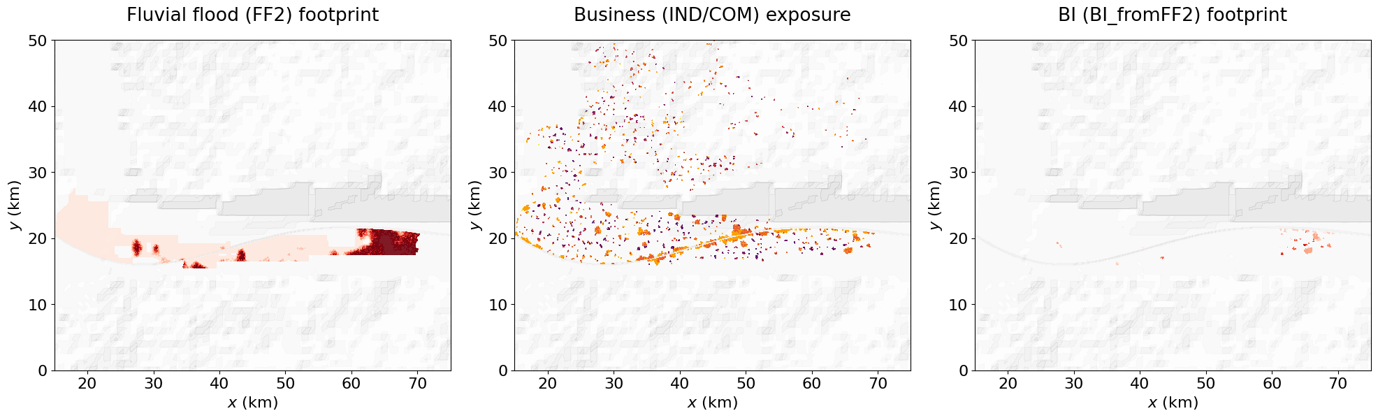
C.6.2. BO to BI
The next code cell calculates BI from the previously defined BO footprint (see Section C.5, must already be run). This is to be considered a proof-of-concept where BI is caused by lack of served power.
## triggger ##
load_node_served_BO = node_served_BO[indL]
if period == 'day':
    load_node_demand = socioecoLayer.node_demand_day
    block_demand = socioecoLayer.demand_day
else:
    load_node_demand = socioecoLayer.node_demand_night
    block_demand = socioecoLayer.demand_night

### Business exposure ##
expo_biz = socioecoLayer.O
load_ID = socioecoLayer.load_ID

## footprint of BI triggered by BO ##
BI_fromBO_fp_yr = GenMR_perils.calc_BI_from_BO(load_node_served_BO, load_node_demand, load_ID, \
                                               expo_biz, block_demand)
duration_BO_da = GenMR_perils.calc_BI_duration_fromBO(g_intact, g_dmg, g_BO, src.par['BI'])
BI_fromBO_fp = BI_fromBO_fp_yr * duration_BO_da / 365.


## plot ##
plt.rcParams['font.size'] = 16
fig, ax = plt.subplots(1,3, figsize=(20, 7))
xmin_BI, xmax_BI, ymin_BI, ymax_BI = 15, 70, 15, 65

fraction_unacceptable = .1
fraction_served = (node_served_BO[indL] - node_demand[indL])/node_demand[indL]

load_col_BO = np.array([
    'black' if name in BO_loads else
    'red' if fraction_served[i] < -fraction_unacceptable else
    'darkorange' if fraction_served[i] < -1e-6 else
    'green'
    for i, name in enumerate(load_nodes)
])

ax[0].contourf(grid.xx, grid.yy, GenMR_env.ls.hillshade(topoLayer.z, vert_exag = .1), cmap = 'gray', alpha = .1)
for (i,j), color, w in zip(edges, edge_col_BO, edge_width_BO):
    x = [node_coords[i,0], node_coords[j,0]]
    y = [node_coords[i,1], node_coords[j,1]]
    ax[0].plot(x, y, color=color, linewidth=w)
for i, c, s in zip(indL, load_col_BO, load_s_BO):
    ax[0].scatter(node_coords[i,0], node_coords[i,1], color=c, s=s, zorder=2)
ax[0].set_xlabel('$x$ (km)')
ax[0].set_ylabel('$y$ (km)')
ax[0].set_title(f'Blackout footprint during {period}', pad = 10)
ax[0].set_aspect(1)
ax[0].set_xlim(xmin_BI, xmax_BI)
ax[0].set_ylim(ymin_BI, ymax_BI)

n_colors = 10
color_indices = np.array(socioecoLayer.load_ID) % n_colors
color_indices[np.isnan(socioecoLayer.load_ID)] = np.nan
ax[1].contourf(grid.xx, grid.yy, GenMR_env.ls.hillshade(topoLayer.z, vert_exag=.1), cmap='gray', alpha = .1)
ax[1].pcolormesh(grid.xx, grid.yy, color_indices, cmap='tab10', alpha = .2)
ax[1].contourf(grid.xx, grid.yy, expo_biz, cmap = 'inferno_r', alpha = 1)
load_coords = node_coords[indL]
ax[1].scatter(load_coords[:,0], load_coords[:,1], color = 'black', s = 10)
ax[1].set_xlabel('$x$ (km)')
ax[1].set_ylabel('$y$ (km)')
ax[1].set_title('Power supply ID', pad = 10)
ax[1].set_xlim(xmin_BI, xmax_BI)
ax[1].set_ylim(ymin_BI, ymax_BI)
ax[1].set_aspect(1)

ax[2].contourf(grid.xx, grid.yy, GenMR_env.ls.hillshade(topoLayer.z, vert_exag=.1), cmap='gray', alpha = .1)
ax[2].contourf(grid.xx, grid.yy, BI_fromBO_fp, cmap = 'Reds', alpha = 1)
ax[2].set_xlabel('$x$ (km)')
ax[2].set_ylabel('$y$ (km)')
ax[2].set_title('BI (BI_fromBO) footprint', pad = 20)
ax[2].set_aspect(1)
ax[2].set_xlim(xmin_BI, xmax_BI)
ax[2].set_ylim(ymin_BI, ymax_BI)

plt.tight_layout();

print('Total BI (Bn. EUR):', np.round(np.nansum(BI_fromBO_fp) * 1e-9, decimals = 2))
print('Total BI duration (da):', np.round(duration_BO_da))
Total BI (Bn. EUR): 1.3
Total BI duration (da): 5.0
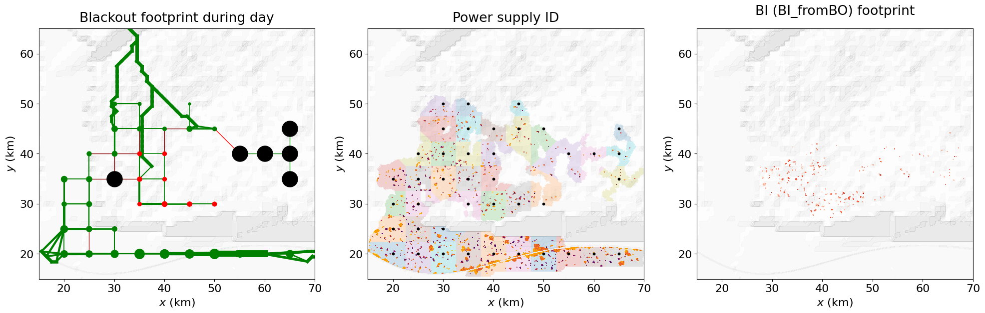
C.7. Public safety service case
A footprint is computed given the fluvial flood event FF2_fromRS2. The approach is identical to BI modelling (see section C.6.1) but with a different damage threshold. The final value, i.e. the percentage of service lost, will be used as input parameter for social unrest (SU) modelling (see Section C.8).
## triggger ##
FF2_fp_dmg = catalog_dmgFootprints['FF_fromRS2']

# correct for building height - TO DO: move this to FF damage assessment function...
h_story = 3.                                    # m per storey
H_bldg = urbLandLayer.bldg_Nstories * h_story   # (m) to move to urbLandLayer class...
h_FF = catalog_dynhazFootprints['FF_fromRS2']  # flood depth (m)
flood_fraction = np.minimum(1., h_FF / H_bldg )
FF2_fp_dmg = FF2_fp_dmg * flood_fraction


## Sf locs triggered by FF2 flood ##
Sf_hosp, Sf_pol, Sf_fire, hosp_OFF, pol_OFF, fire_OFF = GenMR_perils.calc_Sf(socioecoLayer, \
                                                                             src.par['Sf'], FF2_fp_dmg)

## plot ##
plt.rcParams['font.size'] = 16
fig, ax = plt.subplots(1, 3, figsize=(20, 7))
xmin_BI, xmax_BI, ymin_BI, ymax_BI = 15, 75, 0, 50

ax[0].contourf(grid.xx, grid.yy, GenMR_env.ls.hillshade(topoLayer.z, vert_exag=.1), cmap='gray', alpha = .1)
ax[0].contourf(grid.xx, grid.yy, FF2_fp_dmg, cmap = 'Reds', vmin=0, vmax=1, alpha = .9)
ax[0].set_xlabel('$x$ (km)')
ax[0].set_ylabel('$y$ (km)')
ax[0].set_title('Fluvial flood (FF2) footprint', pad = 20)
ax[0].set_aspect(1)
ax[0].set_xlim(xmin_BI, xmax_BI)
ax[0].set_ylim(ymin_BI, ymax_BI)

ax[1].contourf(grid.xx, grid.yy, GenMR_env.ls.hillshade(topoLayer.z, vert_exag=.1), cmap='gray', alpha = .1)
ax[1].scatter(socioecoLayer.hosp_coords[:,0], socioecoLayer.hosp_coords[:,1], color = 'blue', \
              marker = 's', label = 'hospital')
ax[1].scatter(socioecoLayer.pol_coords[:,0], socioecoLayer.pol_coords[:,1], color = 'black', \
              marker = '.', label = 'police')
ax[1].scatter(socioecoLayer.fire_coords[:,0], socioecoLayer.fire_coords[:,1], color = 'red', \
              marker = '+', label = 'fire sta.')
ax[1].set_xlabel('$x$ (km)')
ax[1].set_ylabel('$y$ (km)')
ax[1].set_title('Public safety facilities', pad = 20)
ax[1].set_aspect(1)
ax[1].set_xlim(xmin_BI, xmax_BI)
ax[1].set_ylim(ymin_BI, ymax_BI)

ax[2].contourf(grid.xx, grid.yy, GenMR_env.ls.hillshade(topoLayer.z, vert_exag=.1), cmap='gray', alpha = .1)
ax[2].scatter(socioecoLayer.hosp_coords[hosp_OFF,0], socioecoLayer.hosp_coords[hosp_OFF,1], color = 'blue', \
              marker = 's', label = 'hospital')
ax[2].scatter(socioecoLayer.pol_coords[pol_OFF,0], socioecoLayer.pol_coords[pol_OFF,1], color = 'black', \
              marker = '.', label = 'police')
ax[2].scatter(socioecoLayer.fire_coords[fire_OFF,0], socioecoLayer.fire_coords[fire_OFF,1], color = 'red', \
              marker = '+', label = 'fire sta.')
ax[2].set_xlabel('$x$ (km)')
ax[2].set_ylabel('$y$ (km)')
ax[2].set_title('Sf (Sf_fromFF2) footprint', pad = 20)
ax[2].set_aspect(1)
ax[2].set_xlim(xmin_BI, xmax_BI)
ax[2].set_ylim(ymin_BI, ymax_BI)

plt.tight_layout();


print('Hospital service loss percentage:', Sf_hosp)
print('Police service loss percentage:', Sf_pol)
print('Fire service loss percentage:', Sf_fire)
Hospital service loss percentage: 2.02
Police service loss percentage: 3.28
Fire service loss percentage: 2.53
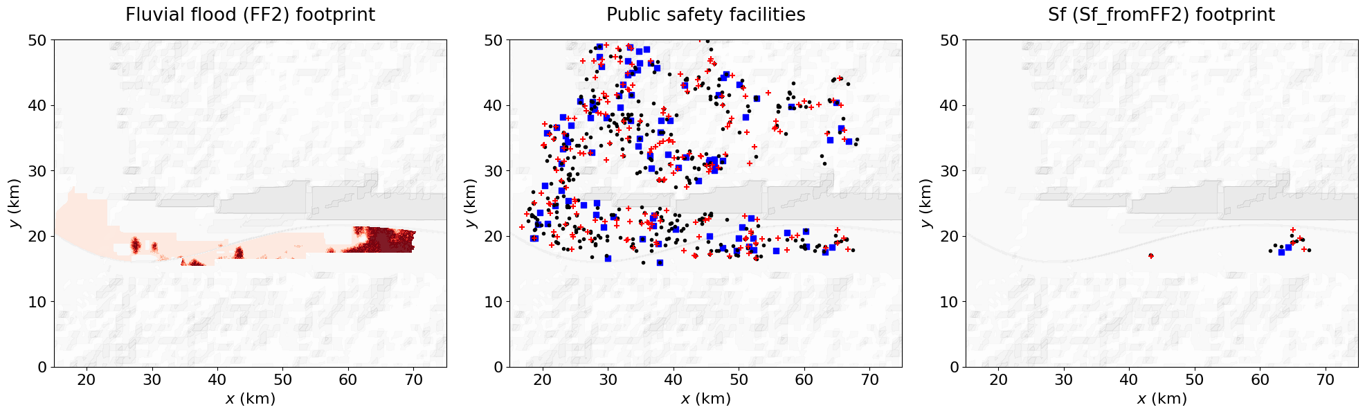
C.8. Social unrest case
Social unrest (SU) is a secondary peril defined as follows:
Source: Triggered by a high level of grievance \(G\), which increases according to Maslow’s Hierarchy of Needs. The following components are amplified for lower wealth levels:
Loss of ‘esteem’ (\(G1\)): Defined as loss of job (via
BIduration);Loss of ‘safety’ (\(G2\)): Defined as lack of access to public services (via
Sf);Loss of ‘physiological needs’ (\(G3\)): Defined as lack of food (i.e., crop BI or no external supply).
Intensity footprints:
Seed event (threshold based): A seed SU event occurs at (x,y) once the grievance threshold has been reached.
Propagated event (threshold based): The seed event expands as more BI is triggered by arson
Damage footprints: Damage occurs by fire (arson) to commercial (COM) blocks at the vicinity of unrest areas.
C.8.1. Generate seed event
scenario = 'BOtrigger'  # 'FFtrigger' or 'BOtrigger' for testing

if scenario == 'FFtrigger':
    BIduration_fp = BI_fromFF2_duration
    BI_fp = BI_fromFF2_fp

    Sf_off = [hosp_OFF, pol_OFF, fire_OFF]
    food_scarcity = 0.  #no food for entire region if 1 (if tot. crops fail, .09 max assuming no additional import)
if scenario == 'BOtrigger':
    BIduration_fp = np.zeros_like(BI_fromBO_fp)
    BIduration_fp[BI_fromBO_fp > 0] = duration_BO_da
    BI_fp = BI_fromBO_fp
    # no Sf event only from BO (backup power)
    Sf_off = [np.zeros(len(socioecoLayer.hosp_coords), dtype=bool), \
              np.zeros(len(socioecoLayer.pol_coords), dtype=bool), \
              np.zeros(len(socioecoLayer.fire_coords), dtype=bool)]
    food_scarcity = 0.01  # for testing


SU0_fp, map_G1, map_G2, map_G3, map_jobloss, map_Sf, map_foodloss = \
    GenMR_perils.calc_SU_seed(BIduration_fp, Sf_off, food_scarcity, socioecoLayer, src.par['SU'])


xmin, xmax, ymin, ymax = 15,70, 15,55
vmax = .5   # amplify to better see low G values

plt.rcParams['font.size'] = '16'
fig, ax = plt.subplots(3,3, figsize=(20,14))

ax[0,0].contourf(grid.xx, grid.yy, GenMR_env.ls.hillshade(topoLayer.z, vert_exag=.1), cmap='gray', alpha = .1)
ax[0,0].contourf(grid.xx, grid.yy, map_jobloss, cmap='Reds', alpha = .8, vmin = 0, vmax = 1)
ax[0,0].set_xlabel('$x$ (km)')
ax[0,0].set_ylabel('$y$ (km)')
ax[0,0].set_title('job loss map', pad = 10)
ax[0,0].set_xlim(xmin, xmax)
ax[0,0].set_ylim(ymin, ymax)
ax[0,0].set_aspect(1)

ax[0,1].contourf(grid.xx, grid.yy, GenMR_env.ls.hillshade(topoLayer.z, vert_exag=.1), cmap='gray', alpha = .1)
ax[0,1].contourf(grid.xx, grid.yy, map_G1, cmap='Reds', alpha = .8, vmin = 0, vmax = vmax)
ax[0,1].set_xlabel('$x$ (km)')
ax[0,1].set_ylabel('$y$ (km)')
ax[0,1].set_title('G1 map', pad = 10)
ax[0,1].set_xlim(xmin, xmax)
ax[0,1].set_ylim(ymin, ymax)
ax[0,1].set_aspect(1)

ax[0,2].axis('off')

ax[1,0].contourf(grid.xx, grid.yy, GenMR_env.ls.hillshade(topoLayer.z, vert_exag=.1), cmap='gray', alpha = .1)
ax[1,0].contourf(grid.xx, grid.yy, map_Sf, cmap='Reds', alpha = .8, vmin = 0, vmax = 1)
ax[1,0].set_xlabel('$x$ (km)')
ax[1,0].set_ylabel('$y$ (km)')
ax[1,0].set_title('Public safety service loss map', pad = 10)
ax[1,0].set_xlim(xmin, xmax)
ax[1,0].set_ylim(ymin, ymax)
ax[1,0].set_aspect(1)

ax[1,1].contourf(grid.xx, grid.yy, GenMR_env.ls.hillshade(topoLayer.z, vert_exag=.1), cmap='gray', alpha = .1)
ax[1,1].contourf(grid.xx, grid.yy, map_G2, cmap='Reds', alpha = .8, vmin = 0, vmax = vmax)
ax[1,1].set_xlabel('$x$ (km)')
ax[1,1].set_ylabel('$y$ (km)')
ax[1,1].set_title('G2 map', pad = 10)
ax[1,1].set_xlim(xmin, xmax)
ax[1,1].set_ylim(ymin, ymax)
ax[1,1].set_aspect(1)

ax[1,2].axis('off')

ax[2,0].contourf(grid.xx, grid.yy, GenMR_env.ls.hillshade(topoLayer.z, vert_exag=.1), cmap='gray', alpha = .1)
ax[2,0].contourf(grid.xx, grid.yy, map_foodloss, cmap='Reds', alpha = .8, vmin = 0, vmax = 1)
ax[2,0].set_xlabel('$x$ (km)')
ax[2,0].set_ylabel('$y$ (km)')
ax[2,0].set_title('Lack of food', pad = 10)
ax[2,0].set_xlim(xmin, xmax)
ax[2,0].set_ylim(ymin, ymax)
ax[2,0].set_aspect(1)

ax[2,1].contourf(grid.xx, grid.yy, GenMR_env.ls.hillshade(topoLayer.z, vert_exag=.1), cmap='gray', alpha = .1)
ax[2,1].contourf(grid.xx, grid.yy, map_G3, cmap='Reds', alpha = .8, vmin = 0, vmax = vmax)
ax[2,1].set_xlabel('$x$ (km)')
ax[2,1].set_ylabel('$y$ (km)')
ax[2,1].set_title('G3 map', pad = 10)
ax[2,1].set_xlim(xmin, xmax)
ax[2,1].set_ylim(ymin, ymax)
ax[2,1].set_aspect(1)

ax[2,2].contourf(grid.xx, grid.yy, GenMR_env.ls.hillshade(topoLayer.z, vert_exag=.1), cmap='gray', alpha = .1)
ax[2,2].contourf(grid.xx, grid.yy, SU0_fp, cmap='Reds', alpha = .8, vmin = 0, vmax = vmax)
ax[2,2].set_xlabel('$x$ (km)')
ax[2,2].set_ylabel('$y$ (km)')
ax[2,2].set_title('Social unrest seed footprint', pad = 10)
ax[2,2].set_xlim(xmin, xmax)
ax[2,2].set_ylim(ymin, ymax)
ax[2,2].set_aspect(1)

plt.tight_layout();
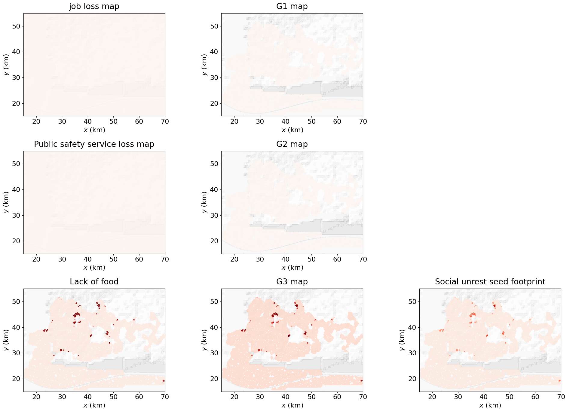
C.8.2. Generate cascading event
if scenario == 'FFtrigger':
    xmin, xmax, ymin, ymax = 66, 70, 17, 22
    src.par['SU']['G_th'] = .2
    src.par['SU']['R_reach_km'] = 3.

elif scenario == 'BOtrigger':
    xmin, xmax, ymin, ymax = 35, 50, 35, 50
    src.par['SU']['G_th'] = .4
    src.par['SU']['R_reach_km'] = 1.


reachable_COM0, SU_buffered0 = GenMR_perils.get_reachable_targets(SU0_fp, BIduration_fp, socioecoLayer, \
                                                                  src.par['SU'])

SU_dmg_fp, SUcasc_fp, BIduration_wSU_fp = \
    GenMR_perils.propagate_SU(SU0_fp, BIduration_fp, Sf_off, food_scarcity, socioecoLayer, src.par, \
                              plt_box = [xmin, xmax, ymin, ymax])

reachable_COM1, SU_buffered1 = GenMR_perils.get_reachable_targets(SUcasc_fp, BIduration_wSU_fp, socioecoLayer, \
                                                                  src.par['SU'])


# tot. SU loss is fire loss on potentially pre-damaged building blocks
SU_t = src.par['SU']['BI2jobloss_mon_th'] * 30.  # days
rebuild_frac = 1. - np.clip((BIduration_fp - SU_t) / BIduration_fp, 0, 1)
L_SU = np.nansum(SU_dmg_fp * urbLandLayer.bldg_blockValue * rebuild_frac)
print('Total SU direct loss (M. EUR):', np.round(L_SU * 1e-6, decimals = 1))

BI_frac = np.clip((BIduration_fp - SU_t) / BIduration_fp, 0, 1)
BI_fp_remaining = BI_fp * BI_frac
BI_fromSU_fp, _ = GenMR_perils.calc_BI_fromDmg(SU_dmg_fp, expo_biz, src.par['BI'])
BI_fp_remaining_noNA = BI_fp_remaining
BI_fp_remaining_noNA[np.isnan(BI_fp_remaining_noNA)] = 0.
BI_fromSU_fp_noNA = BI_fromSU_fp
BI_fromSU_fp_noNA[np.isnan(BI_fromSU_fp_noNA)] = 0.
BI_SU = BI_fromSU_fp_noNA - BI_fp_remaining_noNA
BI_SU[BI_SU < 0.] = 0.
print('Total SU BI (M. EUR):', np.round(np.nansum(BI_SU) * 1e-6, decimals = 1))

plt.rcParams['font.size'] = '16'
fig, ax = plt.subplots(1,2, figsize=(20,10))

SU0_plt = np.full_like(SU0_fp, np.nan)
SU0_plt[SU0_fp >= src.par['SU']['G_th']] = 1
reachable_COM0_plt = reachable_COM0.astype(float)
reachable_COM0_plt[reachable_COM0_plt == 0] = np.nan
ax[0].pcolormesh(grid.xx, grid.yy, urbLandLayer.S, cmap=GenMR_utils.col_S,vmin=-1,vmax=7,alpha=.2,zorder=1)
ax[0].pcolormesh(grid.xx, grid.yy, SU_buffered0.astype(int), cmap='Reds',vmin=0,vmax=10,alpha=.5, zorder=2)
ax[0].pcolormesh(grid.xx, grid.yy, SU0_plt, cmap='Greys', vmin = 0, vmax = 1, zorder = 3)
ax[0].pcolormesh(grid.xx, grid.yy, reachable_COM0_plt, cmap = 'Greens', vmin=0, vmax=2, zorder = 4)
ax[0].set_xlabel('$x$ (km)')
ax[0].set_ylabel('$y$ (km)')
ax[0].set_title('SU seed footprint', pad = 10)
ax[0].set_xlim(xmin, xmax)
ax[0].set_ylim(ymin, ymax)
ax[0].set_aspect(1)

SUcasc_plt = np.full_like(SUcasc_fp, np.nan)
SUcasc_plt[SUcasc_fp >= src.par['SU']['G_th']] = 1
SU_dmg_plt = SU_dmg_fp.copy()
SU_dmg_plt[SU_dmg_fp == 0] = np.nan
reachable_COM1_plt = reachable_COM1.astype(float)
reachable_COM1_plt[reachable_COM1_plt == 0] = np.nan
ax[1].pcolormesh(grid.xx, grid.yy, urbLandLayer.S, cmap=GenMR_utils.col_S,vmin=-1,vmax=7,alpha=.2,zorder=1)
ax[1].pcolormesh(grid.xx, grid.yy, SU_buffered1.astype(int), cmap='Reds',vmin=0,vmax=10,alpha=.5, zorder=2)
ax[1].pcolormesh(grid.xx, grid.yy, SUcasc_plt, cmap='Greys', vmin = 0, vmax = 1, zorder = 3)
ax[1].pcolormesh(grid.xx, grid.yy, reachable_COM1_plt, cmap = 'Greens', vmin=0, vmax=2, zorder = 4)
ax[1].pcolormesh(grid.xx, grid.yy, SU_dmg_plt, cmap='Reds', vmin = 0, vmax = 1)
ax[1].set_xlabel('$x$ (km)')
ax[1].set_ylabel('$y$ (km)')
ax[1].set_title('SU final footprint', pad = 10)
ax[1].set_xlim(xmin, xmax)
ax[1].set_ylim(ymin, ymax)
ax[1].set_aspect(1)

plt.tight_layout();
1/5: Cum. number of burned COM blocks = 2.0
2/5: Cum. number of burned COM blocks = 10.0
3/5: Cum. number of burned COM blocks = 16.0
4/5: Cum. number of burned COM blocks = 22.0
5/5: Cum. number of burned COM blocks = 31.0
Total SU direct loss (M. EUR): 185.2
Total SU BI (M. EUR): 600.9